当前位置:网站首页>Summary of learning notes of deep learning application development (II)
Summary of learning notes of deep learning application development (II)
2022-07-25 07:12:00 【Hua Weiyun】
Say : Matrix operations , It is the basic means of machine learning , Must master .
So there is linear algebra 、 Basic introduction of matrix operation .
Scalar is a special vector ( Row vector 、 Column vector ), A vector is a special matrix ; so , Scalar , It is also a special matrix , A row by column matrix .
import numpy as np# Scalar : Single number scalar_value=18print(scalar_value)18print(scalar_value,scalar_value.shape)# stay tf in ,shape Would be () ; python in int No, shape The concept of ---------------------------------------------------------------------------AttributeError Traceback (most recent call last)<ipython-input-3-0eab86f663c9> in <module>----> 1 print(scalar_value,scalar_value.shape)AttributeError: 'int' object has no attribute 'shape'scalar_np=np.array(scalar_value)print(scalar_np,scalar_np.shape)18 ()# vector : An ordered array of numbers vector_value=[1,2,3]vector_np=np.array(vector_value)print(vector_np,vector_np.shape)# One dimensional array , Can't calculate row vectors 、 Nor is it a column vector . Row vector 、 Or column vectors , It should be represented by a two-dimensional array [1 2 3] (3,)# matrix : Ordered two-dimensional array matrix_list=[[1,2,3],[4,5,6]]matrix_np=np.array(matrix_list)print('matrix_list=',matrix_list)print('matrix_np=\n',matrix_np)print('matrix_np.shape=',matrix_np.shape)matrix_list= [[1, 2, 3], [4, 5, 6]]matrix_np= [[1 2 3] [4 5 6]]matrix_np.shape= (2, 3)# Row vector 、 Matrix representation of column vectors vector_row=np.array([[1,2,3]])print(vector_row,'shape=',vector_row.shape)vector_column=np.array([[4],[5],[7]])print(vector_column,'shape=',vector_column.shape)[[1 2 3]] shape= (1, 3)[[4] [5] [7]] shape= (3, 1)# Matrix and scalar operations matrix_b=matrix_np*2print(matrix_b,'shape=',matrix_b.shape)[[ 2 4 6] [ 8 10 12]] shape= (2, 3)# Matrix and matrix addition and subtraction , The matrix size is required to be the same # Matrix and matrix multiplication :#1 Point multiplication 、 Dot product , The matrix size is required to be the same . It will be used in Convolutional Neural Networks . Use the operator * or np.multiply() Method #2 Cross riding , This one is used more ,A The number of columns in a matrix =B The number of rows in a matrix , result C Matrix is (A Row number ,B Number of columns ), example :(2,3)*(3,4)=(2,4). Use np.matmul() Method matrix_a=np.array([[1,2,3], [4,5,6]])matrix_b=np.array([[1,2,3,4], [2,1,2,0], [3,4,1,2]])np.matmul(matrix_a,matrix_b)array([[14, 16, 10, 10], [32, 37, 28, 28]])# Transposition It can be used .T use reshape() Words , Look at the shape , Not necessarily transpose print(matrix_a,'shape=',matrix_a.shape)print(matrix_a.T,'.T shape=',matrix_a.T.shape)[[1 2 3] [4 5 6]] shape= (2, 3)[[1 4] [2 5] [3 6]] .T shape= (3, 2)matrix_c=matrix_a.reshape(3,2)print(matrix_c,'shape=',matrix_c.shape)[[1 2] [3 4] [5 6]] shape= (3, 2) From a human point of view ,12 Characteristic ratio 1 The characteristics are much more complicated ,
But for computers , It doesn't matter .
stay tf in ,12 Realization of linear regression equation of element , Than 1 Realization of linear equation of element , The code is just a little more complex .
This is the advantage of computer .
Just the result of the final training , Why is it all nan, As the teacher said , My face is black ~
%matplotlib notebookimport tensorflow.compat.v1 as tftf.disable_eager_execution()import matplotlib.pyplot as pltimport numpy as npimport pandas as pdfrom sklearn.utils import shuffledf=pd.read_csv('data/boston.csv',header=0)print(df) CRIM ZN INDUS CHAS NOX RM AGE DIS RAD TAX \0 0.00632 18.0 2.31 0 0.538 6.575 65.2 4.0900 1 296 1 0.02731 0.0 7.07 0 0.469 6.421 78.9 4.9671 2 242 2 0.02729 0.0 7.07 0 0.469 7.185 61.1 4.9671 2 242 3 0.03237 0.0 2.18 0 0.458 6.998 45.8 6.0622 3 222 4 0.06905 0.0 2.18 0 0.458 7.147 54.2 6.0622 3 222 .. ... ... ... ... ... ... ... ... ... ... 501 0.06263 0.0 11.93 0 0.573 6.593 69.1 2.4786 1 273 502 0.04527 0.0 11.93 0 0.573 6.120 76.7 2.2875 1 273 503 0.06076 0.0 11.93 0 0.573 6.976 91.0 2.1675 1 273 504 0.10959 0.0 11.93 0 0.573 6.794 89.3 2.3889 1 273 505 0.04741 0.0 11.93 0 0.573 6.030 80.8 2.5050 1 273 PTRATIO LSTAT MEDV 0 15.3 4.98 24.0 1 17.8 9.14 21.6 2 17.8 4.03 34.7 3 18.7 2.94 33.4 4 18.7 5.33 36.2 .. ... ... ... 501 21.0 9.67 22.4 502 21.0 9.08 20.6 503 21.0 5.64 23.9 504 21.0 6.48 22.0 505 21.0 7.88 11.9 [506 rows x 13 columns]df=df.valuesprint(df)[[6.3200e-03 1.8000e+01 2.3100e+00 ... 1.5300e+01 4.9800e+00 2.4000e+01] [2.7310e-02 0.0000e+00 7.0700e+00 ... 1.7800e+01 9.1400e+00 2.1600e+01] [2.7290e-02 0.0000e+00 7.0700e+00 ... 1.7800e+01 4.0300e+00 3.4700e+01] ... [6.0760e-02 0.0000e+00 1.1930e+01 ... 2.1000e+01 5.6400e+00 2.3900e+01] [1.0959e-01 0.0000e+00 1.1930e+01 ... 2.1000e+01 6.4800e+00 2.2000e+01] [4.7410e-02 0.0000e+00 1.1930e+01 ... 2.1000e+01 7.8800e+00 1.1900e+01]]df=np.array(df)print(df)x_data=df[:,:12]y_data=df[:,12]print(x_data,'\n,shape=',x_data.shape)print(y_data,'\n,shape=',y_data.shape) Data omitted ,shape= (506, 12) Data omitted ,shape= (506,)# The data has been read in #None Representing unknown , Because we can bring in one line of samples at a time , You can also bring in multiple lines of samples at one time x=tf.placeholder(tf.float32,[None,12],name='X')y=tf.placeholder(tf.float32,[None,1],name='Y')# Define a namespace with tf.name_scope('Model'): # Initialize random number shape=(12,1) w=tf.Variable(tf.random_normal([12,1],stddev=0.01),name='W') b=tf.Variable(1.0,name='b') def model(x,w,b): return tf.matmul(x,w)+b # Forward prediction pred=model(x,w,b) # This is the advantage of computer . From a human point of view ,12 Variable ratio 1 Variables are a lot more complicated , But for computers , It doesn't matter . The code is just a little more complex .WARNING:tensorflow:From /home/ma-user/anaconda3/envs/TensorFlow-2.1.0/lib/python3.7/site-packages/tensorflow_core/python/ops/resource_variable_ops.py:1635: calling BaseResourceVariable.__init__ (from tensorflow.python.ops.resource_variable_ops) with constraint is deprecated and will be removed in a future version.Instructions for updating:If using Keras pass *_constraint arguments to layers.train_epochs=2learning_rate=0.01# The loss function is still the mean square deviation with tf.name_scope('LossFunction'): loss_function=tf.reduce_mean(tf.pow(y-pred,2)) optimizer=tf.train.GradientDescentOptimizer(learning_rate).minimize(loss_function)# Prepare to carry out sess=tf.Session()init=tf.global_variables_initializer()sess.run(init)for epoch in range(train_epochs): loss_sum=0.0 for xs,ys in zip(x_data,y_data): xs=xs.reshape(1,12) # Deform to be the same as placeholder , Here is a row of samples at a time ys=ys.reshape(1,1) _,loss=sess.run([optimizer,loss_function],feed_dict={x:xs,y:ys}) loss_sum+=loss x_data,y_data=shuffle(x_data,y_data) b0temp=b.eval(session=sess) w0temp=w.eval(session=sess) loss_average=loss_sum/len(y_data) print('epoch=',epoch+1,'loss=',loss_average,'b=',b0temp,'w=',w0temp)epoch= 1 loss= nan b= nan w= [[nan] A little [nan]] The last training did not produce results , All are nan The reason for this has been found ,
It is because the characteristic data is not normalized , What is the concept of normalization ?
Here's a good example , Make a dish ,
Prepare the material duck 、 Bamboo shoot 、… salt 、 The soy sauce … water , Plus cooking heat , Can make a dish .
Every element of cooking above , Can be regarded as a characteristic variable , And weight can be regarded as the value of characteristic variable , such as
Duck meat xxg,( The characteristic variable is duck , The value is xxg)
Bamboo shoot xxg,
…
salt xxg,
water xxg,
Here, the value of the characteristic variable is different in magnitude , For example, water and salt ,
Water can 50g Bits are adjusted by adding and subtracting ,
But salt cannot , If salt with 50g Adjust for unit , Then die of salt immediately , This dish is useless ,
Only with 1g Adjust for unit . In turn, , If the amount of water is 1g To adjust , That man is bored to death .
After normalization , Water and salt are on the same order , The above will not happen .
Through this example , You probably know why to normalize
Then how to normalize , The method is simple , Namely
( The eigenvalue - The smallest eigenvalue )/( Maximum eigenvalue - The smallest eigenvalue )
The normalized value , The scope is [0,1] Between .
The tag value does not need to be normalized
Put the modified code , And the results of the training :
# Normalization , Pair column index yes 0 To 11 The eigenvalue of is normalized # Column index yes 12 Is the tag value , There is no need to normalize for i in range(12): df[:,i]= (df[:,i] - df[:,i].min()) / (df[:,i].max() - df[:,i].min())x_data=df[:,:12]y_data=df[:,12]print(x_data,'\n,shape=',x_data.shape)print(y_data,'\n,shape=',y_data.shape)[[0.00000000e+00 1.80000000e-01 6.78152493e-02 ... 2.08015267e-01 2.87234043e-01 8.96799117e-02] Data omitted [4.61841693e-04 0.00000000e+00 4.20454545e-01 ... 1.64122137e-01 8.93617021e-01 1.69701987e-01]] ,shape= (506, 12)[24. 21.6 34.7 33.4 36.2 28.7 22.9 27.1 16.5 18.9 15. 18.9 21.7 20.4 Data omitted 22. 11.9] ,shape= (506,)train_epochs=5learning_rate=0.01# The loss function is still the mean square deviation with tf.name_scope('LossFunction'): loss_function=tf.reduce_mean(tf.pow(y-pred,2)) optimizer=tf.train.GradientDescentOptimizer(learning_rate).minimize(loss_function)# Prepare to carry out sess=tf.Session()init=tf.global_variables_initializer()sess.run(init)for epoch in range(train_epochs): loss_sum=0.0 for xs,ys in zip(x_data,y_data): xs=xs.reshape(1,12) # Deform to be the same as placeholder , Here is a row of samples at a time ys=ys.reshape(1,1) _,loss=sess.run([optimizer,loss_function],feed_dict={x:xs,y:ys}) loss_sum+=loss x_data,y_data=shuffle(x_data,y_data) b0temp=b.eval(session=sess) w0temp=w.eval(session=sess) loss_average=loss_sum/len(y_data) print('epoch=',epoch+1,'loss=',loss_average,'b=',b0temp,'w=',w0temp)epoch= 1 loss= 76.95622714730456 b= 15.579174 w= [[-1.7869571 ] Data omitted [-5.5532546 ]]epoch= 5 loss= 27.729550849818775 b= 18.857027 w= [[ -3.5491831] Data omitted [-15.602908 ]] ran 5 round , There will be no more nan 了 .
Losses are still slowly declining , So there is still room to continue running to reduce losses .
After the training model came out , To use , But we have no data , Because the data are all used for training .
So in the course , Randomly select a training data to apply to the model .
It's not good , Because it's like asking you to do all the exam questions during learning and training , It's not fair to let you take another exam , Similar to cheating .
It should be to test your knowledge , Let's do something we haven't done .
What about the better way , There are some data , Divide these data ,
Most of them do training 、 A small part is verified 、 Do the test in a small part .
The following is the model application , That is, the predicted code
n=np.random.randint(506)print(n)x_test=x_data[n]x_test=x_test.reshape(1,12)predict=sess.run(pred,feed_dict={x:x_test})print('predict:%f'%predict)target=y_data[n]print('actual:%f'%target)449predict:28.840622actual:31.500000Talk the talk , This is just a teaching demonstration , It is thousands of miles away from the practicality of house price prediction ~
Visualization is still quite important , Because the data can be seen on the graph , It's more intuitive , It is more in line with people's cognitive thinking .
Let's show it first loss Visualization .
use matplot Draw the list values , The call is very simple plt.plot(loss_list)
Abscissa is the index in the list , The ordinate is the list value , That is to say loss value .
You can see , The curve is converging , There's still room for descent , But the space is getting smaller and smaller , It's getting more and more difficult to dig out a little ,
So I can stop there , run 10 The wheel won't run .
The code is as follows :
plt.plot(loss_list)[<matplotlib.lines.Line2D at 0x7f6da8521c50>]
print(loss_list)[77.82311354303044, 39.53100916880596, 32.78715717594304, 30.24906668426993, 28.538294685825065, 26.90825543845976, 26.615498589579083, 26.093776806913393, 25.747446659085497, 25.427977377308565] The example of house price prediction is basically over , The following is to use TensorBoard To put the algorithm , And some information of the model training process .
Visualization is a matter of opinion , Contribute to the understanding and promotion of information .
Visualization in modelarts Under the old training assignment ,
Is the charge , But this service is no longer available in the new version of the training assignment ,
OK, because the use of this visual service is not very active
So in Modelarts It's not convenient to do this visualization in the product , But that's okay , We can use another cloud product to do , Namely cloudide
House price tf2 edition , There are some changes .
- Direct use sklearn.preprocessing Inside scale To do normalization , It's simpler and more convenient
- Not all the data is used for training , It is divided into two parts for training 、 verification 、 Test data
- Loss function , On the optimizer side , Code changes , Have a headache ~
- There is no operation to break up the training data
The code is as follows :
Last loss It looks big , It's over a hundred , It's because it's squared ~ I guess
%matplotlib inlineimport tensorflow as tfimport matplotlib.pyplot as pltimport numpy as npimport pandas as pdfrom sklearn.utils import shufflefrom sklearn.preprocessing import scaledf=pd.read_csv('data/boston.csv',header=0)#print(df.describe())#print(df)df.head(3)| CRIM | ZN | INDUS | CHAS | NOX | RM | AGE | DIS | RAD | TAX | PTRATIO | LSTAT | MEDV | |
|---|---|---|---|---|---|---|---|---|---|---|---|---|---|
| 0 | 0.00632 | 18.0 | 2.31 | 0 | 0.538 | 6.575 | 65.2 | 4.0900 | 1 | 296 | 15.3 | 4.98 | 24.0 |
| 1 | 0.02731 | 0.0 | 7.07 | 0 | 0.469 | 6.421 | 78.9 | 4.9671 | 2 | 242 | 17.8 | 9.14 | 21.6 |
| 2 | 0.02729 | 0.0 | 7.07 | 0 | 0.469 | 7.185 | 61.1 | 4.9671 | 2 | 242 | 17.8 | 4.03 | 34.7 |
df=df.values#print(df)df=np.array(df)# Normalization , Pair column index yes 0 To 11 The eigenvalue of is normalized # Column index yes 12 Is the tag value , There is no need to normalize x_data=df[:,:12]y_data=df[:,12]#print(x_data,'\n,shape=',x_data.shape)#print(y_data,'\n,shape=',y_data.shape)train_num=300valid_num=100test_num=len(x_data)-train_num-valid_num# Training set x_train=x_data[:train_num]y_train=y_data[:train_num]# Verification set x_valid=x_data[train_num:train_num+valid_num]y_valid=y_data[train_num:train_num+valid_num]# Test set x_test=x_data[train_num+valid_num:len(x_data)]y_test=y_data[train_num+valid_num:len(x_data)]print(x_train.shape,x_valid.shape,x_test.shape)print(y_train.shape,y_valid.shape,y_test.shape)(300, 12) (100, 12) (106, 12)(300,) (100,) (106,)# Change the type ,sklearn.preprocessing Inside scale The method can be normalized directly x_train=tf.cast(scale(x_train),dtype=tf.float32)x_valid=tf.cast(scale(x_valid),dtype=tf.float32)x_test=tf.cast(scale(x_test),dtype=tf.float32)#None Representing unknown , Because we can bring in one line of samples at a time , You can also bring in multiple lines of samples at one time #x=tf.placeholder(tf.float32,[None,12],name='X')#y=tf.placeholder(tf.float32,[None,1],name='Y')# Define a namespace with tf.name_scope('Model'): # Initialize random number shape=(12,1) W=tf.Variable(tf.random.normal([12,1],mean=0.0,stddev=0.01),dtype=tf.float32) B=tf.Variable(tf.zeros(1),dtype=tf.float32) def model(x,w,b): return tf.matmul(x,w)+b # Forward prediction #pred=model(x,w,b) # This is the advantage of computer . From a human point of view ,12 Variable ratio 1 Variables are a lot more complicated , But for computers , It doesn't matter . The code is just a little more complex .train_epochs=5learning_rate=0.01batch_size=10# The loss function is still the mean square deviation with tf.name_scope('LossFunction'): #loss_function=tf.reduce_mean(tf.pow(y-pred,2)) def loss(x,y,w,b): err=model(x,w,b)-y squared_err=tf.square(err) return tf.reduce_mean(squared_err) def grad(x,y,w,b): # Calculate sample data [x,y] In the parameter [w,b] The gradient at the point with tf.GradientTape() as tape: loss_=loss(x,y,w,b) return tape.gradient(loss_,[w,b]) optimizer=tf.keras.optimizers.SGD(learning_rate) #optimizer=tf.train.GradientDescentOptimizer(learning_rate).minimize(loss_function)# Prepare to carry out #sess=tf.Session()#init=tf.global_variables_initializer()#sess.run(init)loss_list_train=[]loss_list_valid=[]total_step=int(train_num/batch_size)for epoch in range(train_epochs): for step in range(total_step): xs=x_train[step*batch_size:(step+1)*batch_size,:] ys=y_train[step*batch_size:(step+1)*batch_size] grads=grad(xs,ys,W,B) optimizer.apply_gradients(zip(grads,[W,B])) loss_train=loss(x_train,y_train,W,B).numpy() loss_valid=loss(x_valid,y_valid,W,B).numpy() loss_list_train.append(loss_train) loss_list_valid.append(loss_valid) print('epoch={:3d},train_loss={:.4f},valid_loss={:.4f}'.format(epoch+1,loss_train,loss_valid))epoch= 1,train_loss=297.3062,valid_loss=209.3717epoch= 5,train_loss=104.6808,valid_loss=127.0953plt.xlabel('Epochs')plt.ylabel('Loss')plt.plot(loss_list_train,'blue',label='Train Loss')plt.plot(loss_list_valid,'red',label='Valid Loss')plt.legend(loc=1)<matplotlib.legend.Legend at 0x7f59e8638f10>
print('Test_loss:{:.4f}'.format(loss(x_test,y_test,W,B).numpy()))Test_loss:122.4169n=np.random.randint(test_num)y_pred=model(x_test,W,B)[n] #x_test:shape(106,12) W:shape(12,1) Equivalent to all the calculations y_predit=tf.reshape(y_pred,()).numpy()target=y_test[n]print('House id',n,'Actual value',target,'predict value',y_predit)House id 78 Actual value 14.6 predict value 25.130033 Finally, I took a step , I saw it MNIST Handwritten digit recognition , Use a neuron .
MNIST The data set comes from NIST National Institute of standards and technology .
Find handwritten by students and staff .
scale : Training set 55000, Verification set 5000, Test set 10000. The size is about 10M.
Datasets can be downloaded from the website , meanwhile tf I have integrated this data set .
stay notebook Try it :
%matplotlib inlineimport tensorflow.compat.v1 as tftf.disable_eager_execution()import matplotlib.pyplot as plt#tf2 It can't be used inside tf1.x Method to read MNIST data , There is nothing in the compatibility Library import tensorflow.compat.v1.examples.tutorials.mnist.input_data as input_data---------------------------------------------------------------------------ModuleNotFoundError Traceback (most recent call last)<ipython-input-4-d97a1109d08b> in <module>----> 1 import tensorflow.compat.v1.examples.tutorials.mnist.input_data as input_dataModuleNotFoundError: No module named 'tensorflow.compat.v1.examples'# use tf2 To read data import tensorflow as tfimport matplotlib.pyplot as pltmnist = tf.keras.datasets.mnist(train_images,train_labels),(test_image,test_labels)=mnist.load_data()Downloading data from https://storage.googleapis.com/tensorflow/tf-keras-datasets/mnist.npz11493376/11490434 [==============================] - 1s 0us/step# Whether the subsequent processing is used tf1.x To do it? ? Although a little nondescript , Try it later First explore tf2 Read out the data in .
The data representation of each picture is 28*28=784 A numerical , The type of each value is numpy.uint8,uint8 The range of phi is zero 0-255,
This may be the so-called 256 Bitmap ?
Each picture will have its own label , It means that this picture is a number 0-9 Which of them? .
In addition to reshape Reorganize the image , More interesting
The following is a Notebook Code
print(train_images.shape,train_labels.shape,test_image.shape,test_labels.shape)#60000 In the training set 55000 Training and 5000 Validation of the ;28 and 28 Represents the size of the picture (60000, 28, 28) (60000,) (10000, 28, 28) (10000,)print('image data:',train_images[1])print('image label:',train_labels[1])image data: [[ 0 0 0 0 0 0 0 0 0 0 0 0 0 0 0 0 0 0 0 0 0 0 0 0 0 0 0 0] Data omitted [ 0 0 0 0 0 0 0 0 0 0 0 0 0 0 0 0 0 0 0 0 0 0 0 0 0 0 0 0]]image label: 0# Look at what this picture looks like def plot_image(image): plt.imshow(image.reshape(28,28),cmap='binary') plt.show() plot_image(train_images[1])
# Break in and learn reshape, The overall order remains unchanged , But the syncopation point has changed import numpy as npint_array=np.array([i for i in range(64)])print(int_array)print(int_array.reshape(8,8))print(int_array.reshape(4,16))[ 0 1 2 3 4 5 6 7 8 9 10 11 12 13 14 15 16 17 18 19 20 21 22 23 24 25 26 27 28 29 30 31 32 33 34 35 36 37 38 39 40 41 42 43 44 45 46 47 48 49 50 51 52 53 54 55 56 57 58 59 60 61 62 63][[ 0 1 2 3 4 5 6 7] [ 8 9 10 11 12 13 14 15] [16 17 18 19 20 21 22 23] [24 25 26 27 28 29 30 31] [32 33 34 35 36 37 38 39] [40 41 42 43 44 45 46 47] [48 49 50 51 52 53 54 55] [56 57 58 59 60 61 62 63]][[ 0 1 2 3 4 5 6 7 8 9 10 11 12 13 14 15] [16 17 18 19 20 21 22 23 24 25 26 27 28 29 30 31] [32 33 34 35 36 37 38 39 40 41 42 43 44 45 46 47] [48 49 50 51 52 53 54 55 56 57 58 59 60 61 62 63]]# Look at an interesting , hold 28*28 Reshaped to 14*56. It's like transfiguration ,1 A change 2 individual , But each image information after the change is only half of the original image , Only the information expressed by the image is simple ,# So we can still recognize this as 2 individual 0plt.imshow(train_images[1].reshape(14,56),cmap='binary')plt.show()# Compare plot_image(train_images[1])

Here we talk about the single hot code one-hot, Unique heat code is used to represent label data . I already know that , Tag data is simple , That is to say 0-9 A number in the range .
To tell you the truth, what's the use of solo coding , I really haven't understood . What else is the concept of European space , Are very strange .
# Hot coding example .x=[3,4]tf.one_hot(x,depth=10)<tf.Tensor: shape=(2, 10), dtype=float32, numpy=array([[0., 0., 0., 1., 0., 0., 0., 0., 0., 0.], [0., 0., 0., 0., 1., 0., 0., 0., 0., 0.]], dtype=float32)># One dimensional array A=tf.constant([3,9,22,60,8,9])print(tf.argmax(A).numpy())# Two dimensional array axis Shaft for 0 when , Take the largest value in each column , The length of the result is the number of columns .B=tf.constant([[3,20,33,99,11], [2,99,33,12,3], [14,90,1,3,98]] )print(tf.math.argmax(B,axis=0).numpy())print(tf.math.argmax(B,axis=1).numpy())3[2 1 0 0 2][3 1 4]#numpy Also have argmax() Method import numpy as npC=np.array([[3,20,33,99,11], [2,99,33,12,3], [14,90,1,3,98]])print(np.argmax(C,axis=1))[3 1 4]Representation of probability , A number between zero and one can well represent .
This function is used to convert any value into 0~1 A number between .
From a certain point of view , It seems to have similarities with the normalization of training data .
anyway , Deal with numbers , How can it be done without a few suitable functions .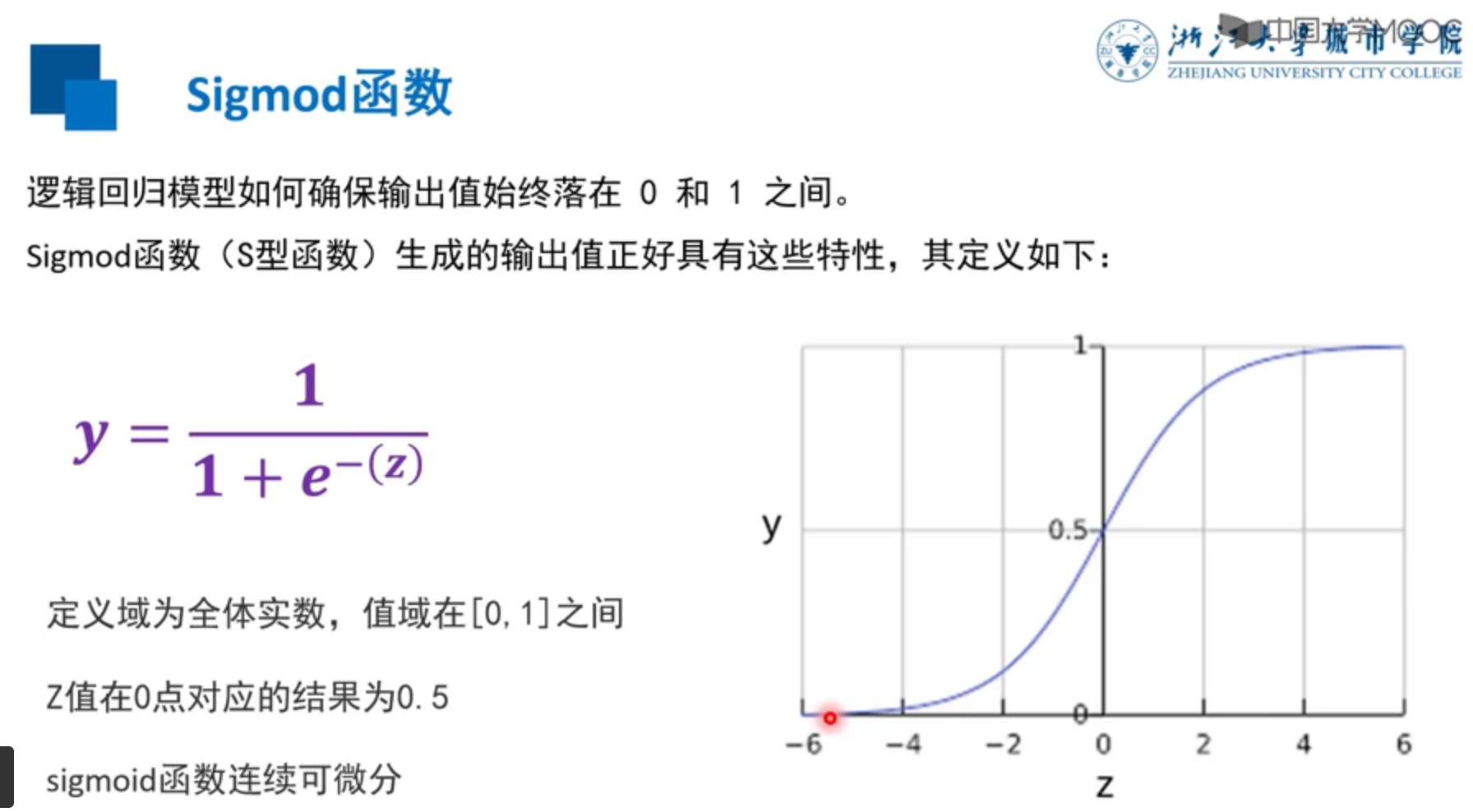
To 2021 year 8 month , I left behind and didn't continue to learn .
边栏推荐
- [Yugong series] July 2022 go teaching course 016 logical operators and other operators of operators
- 2022 Shenzhen cup
- QT6 with vs Code: compiling source code and basic configuration
- js无法获取headers中Content-Disposition
- Talk about practice, do solid work, and become practical: tour the digitalized land of China
- Wechat applet switchtab transmit parameters and receive parameters
- runtimecompiler 和 runtimeonly是什么
- Leetcode 206. reverse linked list I
- 【SemiDrive源码分析】【驱动BringUp】38 - NorFlash & eMMC分区配置
- 流量对于元宇宙来讲并不是最重要的,能否真正给传统的生活方式和生产方式带来改变,才是最重要的
猜你喜欢

2022天工杯CTF---crypto1 wp

With apple not making money, the 2trillion "fruit chain" abandons "fruit" and embraces "special"

Robot engineering - teaching quality - how to judge

Will eating fermented steamed bread hurt your body
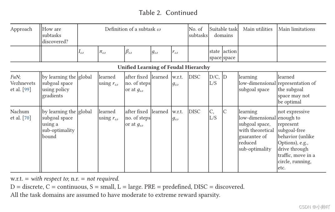
分层强化学习综述:Hierarchical reinforcement learning: A comprehensive survey

Cointelegraph撰文:依托最大的DAO USDD成为最可靠的稳定币

如何在KVM环境中使用网络安装部署多台虚拟服务器

knapsack problem
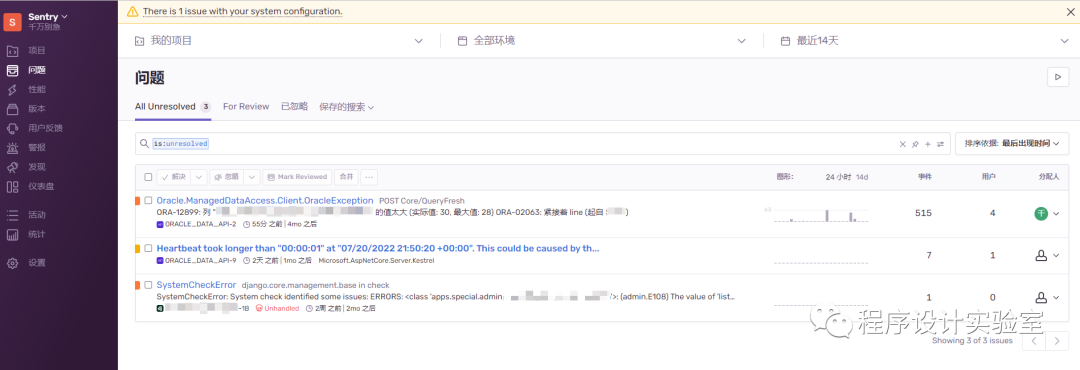
Not only log collection, but also the installation, configuration and use of project monitoring tool sentry

Luo min from qudian, prefabricate "leeks"?
随机推荐
scrapy定时爬虫的思路
The relationship between Informatics, mathematics and Mathematical Olympiad (July 19, 2022) C
流量对于元宇宙来讲并不是最重要的,能否真正给传统的生活方式和生产方式带来改变,才是最重要的
MySQL remote login
[computer explanation] NVIDIA released geforce RTX Super Series graphics cards, and the benefits of game players are coming!
Leetcode118. Yanghui triangle
OpenAtom XuperChain 开源双周报 |2022.7.11-2022.7.22
Go basic notes_ 5_ Process statement
Two week learning results of machine learning
Wechat applet switchtab transmit parameters and receive parameters
微信小程序wx.request接口
10分钟看懂Jmeter 是如何玩转 redis 数据库的
Rongyun launched a real-time community solution and launched "advanced players" for vertical interest social networking
runtimecompiler 和 runtimeonly是什么
[300 + selected interview questions from big companies continued to share] big data operation and maintenance sharp knife interview question column (V)
《游戏机图鉴》:一份献给游戏玩家的回忆录
[Yugong series] July 2022 go teaching course 016 logical operators and other operators of operators
Incremental crawler in distributed crawler
Alibaba cloud image address & Netease cloud image
Vscode saves setting configuration parameters to the difference between users and workspaces