Fourier transform of image

For the principle of Fourier transform, please see Gonzalez and related blogs —— Strangling in Fourier analysis （ Full version ） Updated on 2014.06.06. Because the blogger is not a math major , It can only be explained from the code .

1. Preface

The Fourier transform of the image is from Space domain Change to Spatial frequency domain An operation of . In the frequency domain , We can change the image wave filtering 、 enhance And a series of image processing steps . Compared with image processing in spatial domain , Image processing in frequency domain is relatively simple complex , But the use is more widely . However , People are still unfamiliar with the operation of image Fourier transform , So this paper gives a brief introduction to image Fourier transform , But it does not involve the operation of image processing , Just a brief introduction and demonstration of Fourier Transformation and Reverse transformation The process of , To provide you with a little shallow reference .

The image is Fourier transformed , What you get is a spectrum , The spectrum is consistent with the size of the image , But it contains Space frequency Information about , It is mainly divided into High frequency components and Low frequency component . among , Low frequency component , Also called DC component , Represents the original image Smooth part , It is mainly distributed in the Four corners , Occupying the spectrum Most of the energy , Therefore, the low-frequency components in the spectrum are High brightness ; High frequency components , Also called AC component , Represents the original image Fringe part , It is mainly distributed in the The central , Occupying the spectrum A small amount of energy , Therefore, the low-frequency components in the spectrum are The brightness is very low .

Because the DC component is distributed in four corners , For ease of handling , We usually Move the low-frequency component to the center of the spectrum , And move the high-frequency component to the four corners of the spectrum . The specific operation is shown in the figure below ： Also is to A and D Exchange ,B and C Exchange , This process is Centralization .

The following figure shows an intuitive picture of the spectrum after decentralization and centralization Amplitude spectrum ： You can see , The low frequency component of the centralized amplitude spectrum is located in the center of the image .

If the spectrum is centralized , So when we do the inverse Fourier transform to recover to the spatial domain , It is necessary to centralize the spectrum again （ The two centralizations cancel each other out ）, Then the inverse Fourier transform can change back to the original graph ; If the spectrum of the original image is not centralized , Then we can directly perform inverse Fourier transform on the spectrum . Obvious , The result of the inverse transformation is the same .

2. Code

test_fft.py

import numpy as np
import cv2
import torch.fft

#  Centralization （ Anti centralization ）-->  On the symmetric transformation of the image center .
def FFT_SHIFT(img):
    fimg = img.clone()
    m,n = fimg.shape
    m = int(m / 2)
    n = int(n / 2)

    for i in range(m):
        for j in range(n):
            fimg[i][j] = img[m+i][n+j]
            fimg[m+i][n+j] = img[i][j]
            fimg[m+i][j] = img[i][j+n]
            fimg[i][j+n] = img[m+i][j]

    return fimg

if __name__ == '__main__':
    #  Image Reading 
    pattern = cv2.imread("rectangle.png",0)
    pattern = torch.from_numpy(pattern).type(torch.float32)

    #  Fourier transformation 
    pattern_fft = torch.fft.fftn(pattern)
    pattern_fft_shift = FFT_SHIFT(pattern_fft) #  Centralization 
    pattern_amplitude = torch.log(torch.abs(pattern_fft)) #  Obtain the amplitude spectrum 
    pattern_amplitude_shift = torch.log(torch.abs(pattern_fft_shift))  #  Get the centralized amplitude spectrum 
    pattern_phase = torch.angle(pattern_fft) #  Obtain phase spectrum 
    pattern_phase = pattern_phase - torch.floor(pattern_phase / (2 * np.pi)) * 2 * np.pi
    pattern_phase_shift = torch.angle(pattern_fft_shift)  #  Get the centralized phase spectrum 
    pattern_phase_shift = pattern_phase_shift - torch.floor(pattern_phase_shift / (2 * np.pi)) * 2 * np.pi

    pattern_amplitude = pattern_amplitude.numpy() # torch -> numpy
    pattern_amplitude_shift = pattern_amplitude_shift.numpy()
    pattern_phase = pattern_phase.numpy()
    pattern_phase_shift = pattern_phase_shift.numpy()

    #  Inverse Fourier transform 
    # pattern_ifft = torch.fft.ifftn(pattern_fft) #  The inverse Fourier transform is directly performed on the unfocused spectrum 
    #  Or re centralize the centralized spectrum （ It's called de centralisation ）, Then the inverse Fourier transform 
    pattern_ifft_shift = FFT_SHIFT(pattern_fft_shift) #  Anti centralization 
    pattern_ifft_shift = torch.fft.ifftn(pattern_ifft_shift) #  Inverse Fourier transform 
    pattern_ifft_shift = torch.abs(pattern_ifft_shift) #  The result of the inverse transformation is a complex number , The original image can be obtained only by taking the amplitude 

    pattern_ifft_shift = pattern_ifft_shift.numpy() # torch -> numpy

    #  preservation 
    max_p = np.max(pattern_amplitude)
    min_p = np.min(pattern_amplitude)
    pattern_amplitude = 255.0 * (pattern_amplitude - min_p) / (max_p - min_p)
    pattern_amplitude = pattern_amplitude.astype(np.uint8)
    cv2.imwrite("pattern_amplitude.png",pattern_amplitude) #  Save the amplitude spectrum 
    pattern_amplitude_shift = 255.0 * (pattern_amplitude_shift - min_p) / (max_p - min_p)
    pattern_amplitude_shift = pattern_amplitude_shift.astype(np.uint8)
    cv2.imwrite("pattern_amplitude_shift.png", pattern_amplitude_shift)  #  Save the centralized amplitude spectrum 

    max_p = np.max(pattern_phase)
    min_p = np.min(pattern_phase)
    pattern_phase = 255.0 * (pattern_phase - min_p) / (max_p - min_p)
    pattern_phase = pattern_phase.astype(np.uint8)
    cv2.imwrite("pattern_phase.png",pattern_phase)
    pattern_phase_shift = 255.0 * (pattern_phase_shift - min_p) / (max_p - min_p)
    pattern_phase_shift = pattern_phase_shift.astype(np.uint8)
    cv2.imwrite("pattern_phase_shift.png", pattern_phase_shift) #  Save the centralized phase spectrum 

    pattern_ifft_shift = pattern_ifft_shift.astype(np.uint8)
    cv2.imwrite("pattern_ifft.png",pattern_ifft_shift) #  Save the inverse Fourier transform result 
    

show_image.py

import matplotlib.pyplot as plt
import cv2

plt.rcParams['font.sans-serif'] = ['SimHei'] #  Used to display Chinese labels normally 
plt.rcParams['axes.unicode_minus'] = False #  Used to display negative sign normally 

#  Show results 
if __name__ == '__main__':
    #  Image Reading 
    pattern = cv2.imread("1.png",0)
    pattern_amplitude = cv2.imread("pattern_amplitude.png",0)
    pattern_amplitude_shift = cv2.imread("pattern_amplitude_shift.png",0)
    pattern_phase = cv2.imread("pattern_phase.png", 0)
    pattern_phase_shift = cv2.imread("pattern_phase_shift.png", 0)
    pattern_ifft = cv2.imread("pattern_ifft.png", 0)

    plt.subplot(231),plt.imshow(pattern),plt.title(" Original picture ")
    plt.subplot(232),plt.imshow(pattern_amplitude),plt.title(" Amplitude spectrum ")
    plt.subplot(233),plt.imshow(pattern_phase),plt.title(" Phase spectrum ")
    plt.subplot(234),plt.imshow(pattern_ifft),plt.title(" Inverse Fourier transform ")
    plt.subplot(235),plt.imshow(pattern_amplitude_shift),plt.title(" Centralized amplitude spectrum ")
    plt.subplot(236),plt.imshow(pattern_phase_shift),plt.title(" Centralized phase spectrum ")
    plt.show()
    

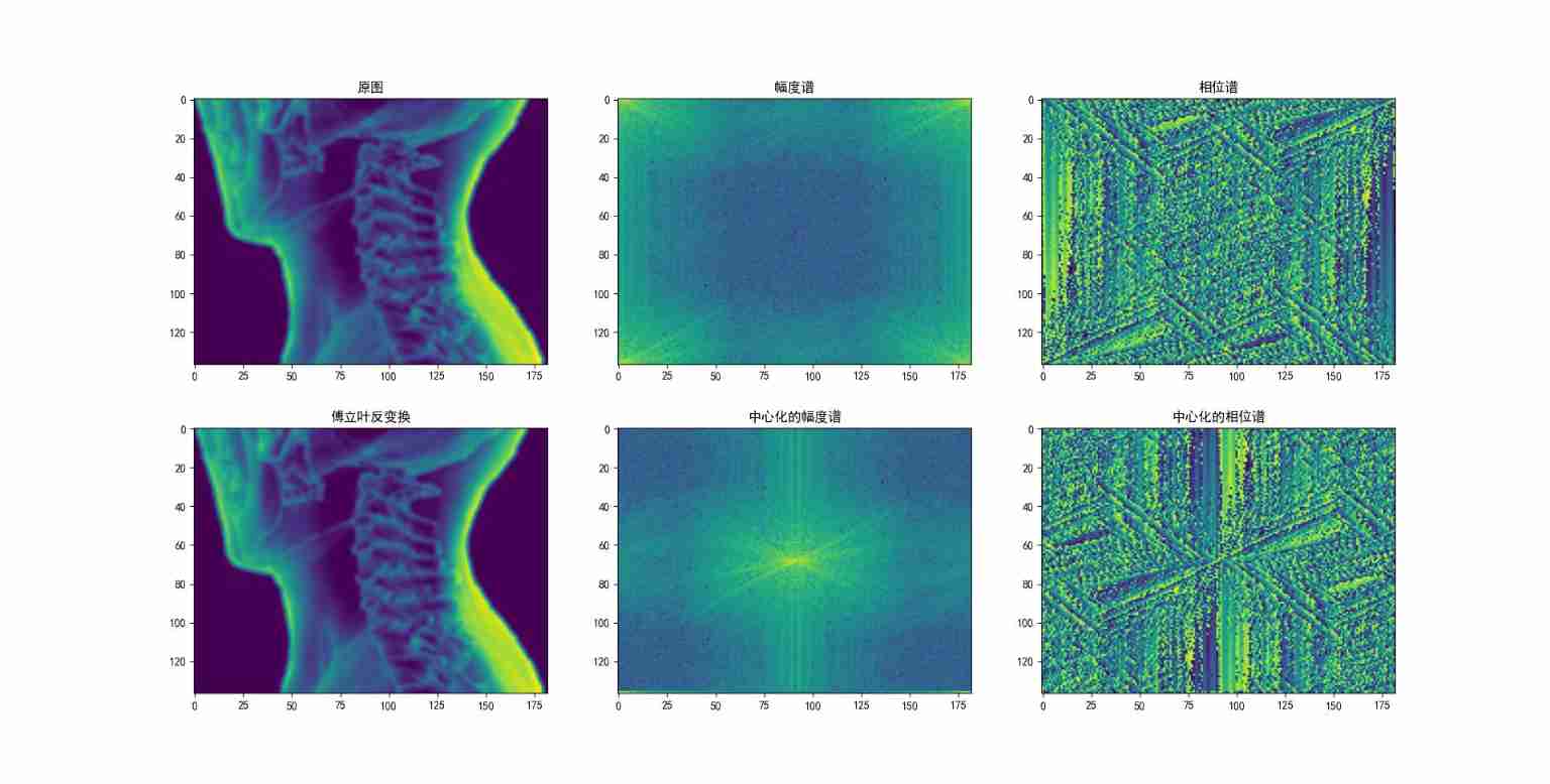
3. Result display

The following shows the results of the three original pictures , The color in the picture is plt default cmap mapping .

4. additional ——numpy.fft Realize Fourier transform

show_image.py

import cv2
import numpy as np
import matplotlib.pyplot as plt

plt.rcParams['font.sans-serif'] = ['SimHei']  #  Used to display Chinese labels normally 
plt.rcParams['axes.unicode_minus'] = False  #  Used to display negative sign normally 

if __name__ == "__main__":
    image = cv2.imread("rectangle.png", 0)
    #  Yes image Do FFT , The output is in the plural form 
    fft = np.fft.fft2(image)
    # np.fft.fftshift Move the zero frequency component to the center of the spectrum 
    fft_shift = np.fft.fftshift(fft)
    #  Take the absolute value , Change the plural form to a real number 
    #  The purpose of absolute value is to change the data to a small range 
    s1 = np.log(np.abs(fft))
    s2 = np.log(np.abs(fft_shift))
    # np.angle The angle can be calculated directly from the imaginary and real parts of the complex number , The default angle is radians 
    phase_f = np.angle(fft)
    phase_f_shift = np.angle(fft_shift)
    print(phase_f)
    #  Inverse Fourier transform 
    ifft_shift = np.fft.ifftshift(fft_shift)
    ifft = np.fft.ifft2(ifft_shift)
    #  What comes out is the plural , Unable to display 
    image_back = np.abs(ifft)
    #  Show 
    plt.subplot(231), plt.imshow(image, 'gray'), plt.title(" Original picture "), plt.xticks([]), plt.yticks([])
    plt.subplot(232), plt.imshow(s1, 'gray'), plt.title(" Before the centralization of the amplitude spectrum "), plt.xticks([]), plt.yticks([])
    plt.subplot(233), plt.imshow(s2, 'gray'), plt.title(" After centring the amplitude spectrum "), plt.xticks([]), plt.yticks([])
    plt.subplot(234), plt.imshow(phase_f, 'gray'), plt.title(" Before the centralization of the phase spectrum "), plt.xticks([]), plt.yticks([])
    plt.subplot(235), plt.imshow(phase_f_shift, 'gray'), plt.title(" After the phase spectrum is centered "), plt.xticks([]), plt.yticks([])
    plt.subplot(236), plt.imshow(image_back, 'gray'), plt.title(" Inverse Fourier transform results "), plt.xticks([]), plt.yticks([])
    plt.show()