当前位置:网站首页>Machine learning notes - convolutional neural network memo list
Machine learning notes - convolutional neural network memo list
2022-06-11 09:08:00 【Sit and watch the clouds rise】
One 、 summary
Tradition CNN Convolutional neural network , Also known as CNN, Is a specific type of neural network , It usually consists of the following layers :

Two 、 The main types of layers
1、Convolution layer (CONV)
Convolution layer (CONV) In scan input  Use the filter that performs the convolution operation . Its super parameters include filter size
  And stride
  . Generated output
  It is called characteristic graph or activation graph .

remarks : The convolution step can also be extended to 1D and 3D situation .
2、Pooling (POOL)
Pooling layer (POOL) It is a down sampling operation , It is usually applied after the convolution layer , It has certain space invariance . especially , The largest and average pool is a special type of pool , Take the maximum and average values respectively .
Maximum pooling : Select the maximum value of the current view for each pool operation

The average pooling : Each pooled operation averages the value of the current view

3、Fully Connected (FC)
Fully connected layer (FC) Run on flattened input , Each of these inputs is connected to all neurons . If there is ,FC Layers usually appear in CNN The end of the architecture , Can be used to optimize the target , For example, class scores .

3、 ... and 、 Filter super parameters
Convolution layer containing filter , It is important to understand the meaning behind its superparameters .
1、Dimensions of a filter
One size is  The filter of shall be used to contain
  The input to the channel is a
  Volume , Its pair size is
  The input of performs convolution And generate a size of
  The output characteristic diagram of ( Also called activation diagram ).

remarks : The size is Of  The application of the filter results in an output size of
  Characteristic graph .
2、Stride
For convolution or pooling , Stride Represents the number of pixels the window moves after each operation .

3、Zero-padding
Zero padding means that  The process of adding zeros to each side of the input boundary . This value can be specified manually , It can also be set automatically by one of the three modes detailed below :

Four 、 Adjust super parameters
1、 Parameter compatibility in convolution layer
By paying attention to Enter the length of the volume size , The length of the filter , Zero fill , Stride , Then the output size of the feature graph along this dimension Given by the following formula :

2、 Understand the complexity of the model
To assess the complexity of the model , It is often useful to determine the number of parameters its schema will have . In a given layer of a convolutional neural network , It is done as follows :

3、 Feel the field
The first  The receptive field of the layer is expressed as
  Region , The first Each pixel of an activation map can “ notice ” Of input . By calling
 layer
 Filter size and
 layer
 And use the Convention
 , You can calculate layers using the following formula
Feeling field of :

In the following example ,,
,


5、 ... and 、 Common activation functions
(1)Rectified Linear Unit
Rectifier linear unit layer (ReLU) It's an activation function  , All elements for volume . It aims to introduce nonlinearity into the network . The following table summarizes its variants :

(2)Softmax
softmax Step can be regarded as a generalized logic function , It takes the fractional vector  As input , And output an output probability vector p∈ R Through the... At the end of the architecture softmax function . The definition is as follows :

6、 ... and 、Object detection
(1) Model type
Yes 3 There are three main types of object recognition algorithms , The nature of their predictions is different . They are described in the following table :

(2)Detection
In the context of object detection , According to whether we just want to locate the object or detect more complex shapes in the image , Use different methods . The following table summarizes the two main :

(3)Intersection over Union(IOU)
The intersection of the Union , Also known as IoU, Is a quantitative prediction bounding box  With the actual bounding box
  A function of the degree of correct positioning . It is defined as :

remarks : We always have IoU∈[0,1]. By convention , If  , Then the predicted bounding box Considered to be quite good .

(4)Anchor boxes
Anchor box is a technique for predicting overlapping bounding boxes . In practice , Allow the network to predict multiple boxes at the same time , Each box prediction is limited to a given set of geometric properties . for example , The first prediction may be a rectangle of a given shape , The second prediction may be another rectangle with different geometry .
(5)Non-max suppression
The non maximum suppression technique aims to remove the overlapping bounding boxes of the same object by selecting the most representative bounding box . After removing all probability predictions below 0.6 Behind the box of , Repeat the following steps with the remaining boxes :
For a given class ,
• step 1: Select the box with the maximum prediction probability .
• step 2: Discard any with IoU⩾0.5 And the previous box .

(6)YOLO
You Only Look Once (YOLO) Is an object detection algorithm that performs the following steps :
step 1: Divide the input image into G×G grid .
The first 2 Step : For each grid cell , Run a forecast yy Of CNN, Its form is as follows :
![\boxed{y=\big[\underbrace{p_c,b_x,b_y,b_h,b_w,c_1,c_2,...,c_p}_{\textrm{repeated }k\textrm{ times}},...\big]^T\in\mathbb{R}^{G\times G\times k\times(5+p)}}](http://img.inotgo.com/imagesLocal/202206/11/202206110859382613_51.gif)
among  Is the probability of detecting an object ,
 ,
, ,
, ,
, Is the property of the detected bounding box ,
 ,...,
,..., Is what is detected
  Class one-hot Express , Is the number of anchor frames .
The first 3 Step : Run a non maximum suppression algorithm to remove any potential duplicate overlapping bounding boxes .

(7)R-CNN
Regions with convolutional neural networks (R-CNN) Is an object detection algorithm , It first segments the image to find the potential related bounding boxes , Then run the detection algorithm to find the most likely objects in these bounding boxes .

remarks : Although the original algorithm is computationally expensive and slow , But the newer architecture makes the algorithm run faster , for example Fast R-CNN and Faster R-CNN.
7、 ... and 、 Face verification and recognition
(1) Model type
The following table summarizes the two main model types :

(2)One Shot Learning
One Shot Learning Is a face verification algorithm , It uses a limited training set to learn the similarity function , This function can quantify the different degrees of two given images . The similarity function applied to two images is usually recorded as  .
.
(3)Siamese Network
Siamese Networks It aims to learn how to encode images , Then quantify the difference between the two images . For a given input image  , Coded output is usually recorded as
  .
.
(4)Triplet loss
Triplet loss  Is based on images A( anchor )、P( just ) and N( negative ) The embedding of triples of represents the calculated loss function . Anchor points and positive examples belong to the same category , Negative cases belong to another category . By calling
  Margin parameter , This loss is defined as follows :


8、 ... and 、 Neurostylistic migration
(1)Motivation
The goal of neurostyle transfer is based on the given content C And given style S Generate the image G.

(2)Activation
At a given layer  in , Activation is marked as
 ![a^{[l]}](http://img.inotgo.com/imagesLocal/202201/03/202201030711251168_58.gif) And it's a dimension
And it's a dimension 
(3)Content cost function
Content cost function  Used to determine the generated image G With the original content image C The difference between . The definition is as follows :
}-a^{[l](G)}|| ^2}](http://img.inotgo.com/imagesLocal/202206/11/202206110859382613_43.gif)
(4)Style matrix
Given layer Style matrix ![G^{[l]}](http://img.inotgo.com/imagesLocal/202206/11/202206110859382613_76.gif) It's a Gram matrix , Each of these elements
It's a Gram matrix , Each of these elements ![G_{kk'}^{[l]}](http://img.inotgo.com/imagesLocal/202206/11/202206110859382613_4.gif) The channel is quantified k and k' The relevance of . It's about activating The definition is as follows :
The channel is quantified k and k' The relevance of . It's about activating The definition is as follows :
![\boxed{G_{kk'}^{[l]}=\sum_{i=1}^{n_H^{[l]}}\sum_{j=1}^{n_w^{[l]}}a_ {ijk}^{[l]}a_{ijk'}^{[l]}}](http://img.inotgo.com/imagesLocal/202206/11/202206110859382613_25.gif)
remarks : The style image and the style matrix of the generated image are respectively recorded as }](http://img.inotgo.com/imagesLocal/202112/24/202112240730340558_5.gif) and
and }](http://img.inotgo.com/imagesLocal/202206/11/202206110859382613_75.gif) .
.
(5)Style cost function
Style cost function  Used to determine the generated image G With style S The difference between . The definition is as follows :
![\boxed{J_{\textrm{style}}^{[l]}(S,G)=\frac{1}{(2n_Hn_wn_c)^2}||G^{[l](S)}-G^{[l](G)}||_F^2=\frac{1}{(2n_Hn_wn_c)^2}\sum_{k,k'=1}^{n_c}\Big(G_{kk'}^{[l](S)}-G_{kk'}^{[l](G)}\Big)^2}](http://img.inotgo.com/imagesLocal/202206/11/202206110859382613_61.gif)
(6)Overall cost function
The overall cost function is defined as a combination of content and style cost functions , By the parameter α,β weighting , As shown below :

remarks : Higher α Values make the model more concerned about content , And the higher β Values make the model more concerned about style.
Nine 、 An architecture that uses computational skills
(1)Generative Adversarial Network
Generative antagonistic network , Also known as GAN, It consists of generative model and discriminant model , The generation model aims to generate the most realistic output , This output will be fed into a discrimination model designed to distinguish the generated image from the real image .

remarks : Use GAN Variant use cases include text to image 、 Music generation and synthesis .
(2)ResNet
ResNet Residual network architecture ( Also known as ResNet) Use residual blocks with a large number of layers , Designed to reduce training errors . The residual block has the following characteristic equation :
![\boxed{a^{[l+2]}=g(a^{[l]}+z^{[l+2]})}](http://img.inotgo.com/imagesLocal/202206/11/202206110859382613_69.gif)
(3)Inception Network
The architecture uses the initial modules , To try different convolutions , To improve its performance through feature diversification . especially , It USES  Convolution techniques to limit the computational burden .
边栏推荐
- ERP体系能帮忙企业处理哪些难题?
- ERP体系的这些优势,你知道吗?
- 19. 删除链表的倒数第 N 个结点
- 企业需要考虑的远程办公相关问题
- 1493. 删掉一个元素以后全为 1 的最长子数组
- CUMT learning diary - theoretical analysis of uCOSII - Textbook of Renzhe Edition
- 【软件】大企业ERP选型的方法
- 86. separate linked list
- Comment l'entreprise planifie - t - elle la mise en oeuvre?
- Is it appropriate to apply silicone paint to American Standard UL 790 class a?
猜你喜欢

openstack详解(二十一)——Neutron组件安装与配置

Create a nodejs based background service using express+mysql

CUMT learning diary - theoretical analysis of uCOSII - Textbook of Renzhe Edition

Matlab r2022a installation tutorial
CUMT学习日记——ucosII理论解析—任哲版教材

shell脚本之sed详解 (sed命令 , sed -e , sed s/ new / old / ... )

MSF给正常程序添加后门
What is the process of en 1101 flammability test for curtains?

【C语言-函数栈帧】从反汇编的角度,剖析函数调用全流程
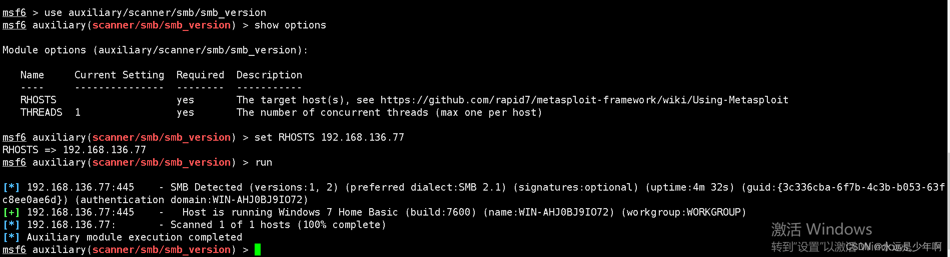
MSF基于SMB的信息收集
随机推荐
【方案开发】红外体温计测温仪方案
Flutter开发日志——路由管理
203. remove linked list elements
C language printing diamond
876. intermediate node of linked list
openstack详解(二十四)——Neutron服务注册
Android 面试笔录(精心整理篇)
[share] how do enterprises carry out implementation planning?
【C语言-函数栈帧】从反汇编的角度,剖析函数调用全流程
Some learning records I=
Screening frog log file analyzer Chinese version installation tutorial
E. Zoom in and zoom out of X (operator overloading)
ERP体系的这些优势,你知道吗?
multiplication table
工厂出产流程中的这些问题,应该怎么处理?
844. compare strings with backspace
206. reverse linked list
Talk about reading the source code
MSF evasion模块的使用
2095. 删除链表的中间节点