Shengxin literature learning (Part1) -- precision: a approach to transfer predictors of drug response from pre-clinical ...

Learning notes , For reference only , If there is a mistake, it must be corrected
Journal：Bioinformatics
Year：2019
Authors：Soufiane Mourragui, Marco Loog, Lodewyk F. A. Wessels

---

---

PRECISE: a domain adaptation approach to transfer predictors of drug response from pre-clinical models to tumors

Abstract

Motivation: Cell lines and patient derived xenotransplantation （PDXs） It has been widely used to understand the molecular basis of cancer . Although core biological processes are usually conservative , But these models also show important differences compared with human tumors , Hinders the transformation of results from preclinical models to the human environment . especially , utilize from pre- clinical The data obtained from the model generate a drug response predictor to predict the patient's response It's still a challenging task . Because it has been pre- clinical The model collects a large number of drug response data sets , The data of patients' drug reactions are often lacking , So there is an urgent need for a method , Change the drug response predictor from pre- clinical The model is effectively transferred to the human environment .

Results: We showed , Cell lines and PDXs It has common characteristics and processes with human tumors . We quantify this similarity , It also shows that the regression model can not be simply applied to cell lines or PDX Training , And then applied to tumors . We developed PRECISE, This is a new method based on domain adaptability , it Captured in a consensus representation pre- clinical Common information between models and human tumors . Using this representation , We are pre- clinical A predictor of drug response trained on data , These predictors were used to stratify human tumors . It turns out that , The resulting domain variable predictor is pre- clinical The prediction performance of the field has decreased slightly , But the important thing is , It reliably restores the known association between independent biomarkers on human tumors and their supporting drugs .

Availability and implementation: PRECISE and the scripts for running our experiments are available on our GitHub page (https://github.com/NKI-CCB/PRECISE).

Introduction

Cancer is a kind of Heterogeneous diseases , As a result of the accumulation of somatic genomic changes . These changes show a high degree of difference between tumors , Resulting in inconsistent response to treatment . Precision medicine attempts to improve the response rate by taking this heterogeneity into account and treating it according to the specific molecular composition of a specific tumor . This requires the identification of biomarkers , To identify a group of patients who will benefit from a particular treatment , And avoid unnecessary side effects for patients who will not benefit . However , Due to the limited patient response data of various drugs ,pre- clinical Pattern , Such as cell line and patient derived xenotransplantation (PDXs) It has been used to generate large-scale data sets , So that personalized treatment strategies based on data-driven response biomarker recognition can be developed . What's more special is , Hundreds pre- clinical The model is not only widely used for molecular characterization , what's more , Their reactions to hundreds of drugs have also been recorded . This leads to a lot of public resources , Including from cell lines （GDSC1000,Iorio wait forsomeone ,2016） and PDX Model （NIBR PDXE,Gao wait forsomeone ,2015） The data of .

these pre- clinical Resources can be used to build predictors of drug response , And then move to the human environment , Allow stratification of medications that the patient has not yet been exposed to . Geeleher By simply correcting the batch effect between cell lines and tumor data sets , Then directly transfer the cell line predictor to the human environment (Geeleher wait forsomeone ,2014,2017). This has produced some promising results ： It restores mature biomarkers , Such as lapatinib sensitivity and ERBB2 The correlation between amplification . However , When the predictor is directly transferred from source domain（ Cell line ） Transferred to the target domain（ Human tumors ） when , We assume that the source and target data come from the same distribution . pre- clinical The differences between models and human tumors have been extensively studied （Ben-David wait forsomeone ,2017,2018;Gillet wait forsomeone ,2013）, The most obvious differences include cell lines and PDXs There is no immune system , And there is no tumor microenvironment and vessel in the cell line . One can therefore not assume similarity between the source and target distributions.

Transfer learning To solve this problem (see Pan and Yang, 2010 for a general review). According to the availability of source and target tags and the specific relationship between these source and target datasets , Transfer learning methods can be classified into different categories . Because we have very few labeled tumor samples , But there are many signs pre- clinical Model , Our approach falls into a category known as transitional [while this terminology is not widely used in the community, we follow the categorization employed in Pan and Yang (2010)]. Due to features （ Genes ） It is the same in the source and target domains , Our problem requires a domain adaptation strategy , It is sometimes called homogeneous domain adaptation .

As mentioned earlier , Preclinical models and tumours marginal distributions Estimates are different . However , We assume that drug reactions are largely caused by pre- clinical The conservative biological phenomena between the model and human tumor . therefore , There should be a set of characteristics ( gene ), For these features , The conditions of drug reaction are distributed in cell lines 、PDXs It is comparable to human tumors . Different approaches have been proposed to find such Common space , These methods can be divided into two categories (Csurka, 2017)：

• The first method , namely data- centric Methods , Can pass aligning the marginal distributions Directly from pre-clinical Model and tumor find a common subspace.
• The second kind of method , be called subspace-centric, By lowering the dimension , then aligning the low-rank representations To modify the domain adaptability (Fernando wait forsomeone ,2013;Gong wait forsomeone ,2012;Gopalan wait forsomeone ,2011).

In the first category , The marginal distribution is directly aligned , This shows that empirical distribution Will fully and accurately reflect source and target samples Of real behavior. for example , If the source dataset ER The proportion of positive samples is very different from the target data set , This direction will be abandoned , Because it is too different between the source and the target . obviously , This is not desirable , Because it represents a very important variable in breast cancer .

The second category found important variations Of directions, And then in source and target Compare these directions . These methods do not directly compare distributions , And it is less affected by the sample size problem and sample selection deviation , therefore , We choose the second method .

We proposed Patient Response Estimation Corrected by Interpolation of Subspace Embeddings (PRECISE), This is an approach based on domain adaptability , Training regression models in the process of sharing human tumors with preclinical models . chart 1 It shows PRECISE General workflow .

We first pass Linear dimensionality reduction From cell lines 、PDXs And human tumors Independent extraction factor . then , Use one Linear transformation , Put one of them pre- clinical Model factors were compared with human tumor factors Geometric matching (Fernando wait forsomeone ,2013). And then we Extract common factors [principal vectors (PVs)], And defined as the direction least affected by linear transformation ( chart 1A).

In choosing the most similar PV after , We do this in the source domain (cell line or PDX PVs) And the target domain (human tumor PVs) Between Interpolation computes a new feature space . The feature space generated by this interpolation allows a balance between the selected model system and the tumor (Gong wait forsomeone ,2012;Gopalan wait forsomeone ,2011). Although this method uses canonical angle The concept of , But it is obviously different from canonical correlation analysis . in fact , In our case , Samples are not paired , Cross correlation cannot be calculated . From a set of Interpolation Spaces , By optimizing the selected pre- clinical The marginal distribution of the model is matched with the human tumor data projected on these interpolation features Consensus means . These consensus features are finally used to train a regression model , Use data from the selected preclinical model . We used this regression model to predict tumor drug response ( chart 1B).

Because these characteristics are shared between preclinical models and human tumors , It is expected that the regression model can be extended to human tumors . Last , We use known biomarkers - Drug Association (from independent data sources, e.g. mutation status, copy number) As a positive control , To verify the prediction results of the model in human tumors ( chart 1C).

Fig. 1. Overview of PRECISE and its validation. (A） Human tumor and preclinical data were first processed independently , To find the most important domain specific factors ( for example PCA). Then compare these factors 、 array , And sort by similarity , produce PVs. first PV Is a pair of vectors that are very similar in geometry , Capture human tumors and pre- clinical Strong commonalities between models , Bottom PV Represents human tumors and pre- clinical The dissimilarity between models . (B) Similar cut-off To be preserved . For the most similar pre- clinical After interpolation between the model and the tumor model , By balancing human tumors with pre- clinical Model , Work out a Consensus means . We analyzed these characteristics Gene set enrichment analysis , To assess their clinical relevance . adopt take pre- clinical And human tumor transcriptomic data projected onto this consensus representation , Finally, a regression model of tumor perception is trained . To test our model , We used positive controls from independent data sources , Such as copy number or mutation data . These positive controls are biomarkers that have been established - Drug Association . We compared the predictions of our model with those based on these independent established biomarkers . The red box highlights our contribution .

This work includes the following new contributions . First , We introduced an extensible 、 Flexible ways to find pre- clinical Common factors between models and human tumors . second , We use this method to quantify cell lines 、PDXs Transcriptional commonalities of biological processes between and human tumors , And we show that these common factors are biologically related . Third , We show how these common factors can be used in regression to predict drug response in human tumors , And we have restored the famous biomarkers - Drug Association . Last , We derive an equivalent 、 faster 、 A more explicable way to calculate geodesic flow kernel, This is a widely used domain adaptation method in computer vision . Our approach is based on Gopalan wait forsomeone （2011 year ） and Gong wait forsomeone （2012 year ） On the basis of our work , But these methods are extended , The first is to automatically remove irrelevant and untransferable information , The second is to find consensus features in the interpolation scheme , To counteract the bias of source characteristics caused by ridge regression .

Materials and methods

Notes on transcriptomics data

We here present the datasets employed in this study. Further notes on preprocessing can be found in Supplementary Subsection 1.3.

The cosine similarity matrix

Transcriptomic data are high dimensional , Yes p ~ 19000 Features （ gene ）, Because these genes are highly correlated , Only some gene combinations are informative . A simple and robust way to find these combinations （Van Der Maaten etc. ,2009） Is to use the linear dimensionality reduction method , Such as principal component analysis （PCA）, Decompose the data matrix into $d_f$ One factor , Used separately for source (cell lines or PDXs) And the target (human tumors), thus ：
$$\forall i\in \{s,t\},X_i=S_i{P}_{i}with{P}_i{P}_i^T=I_{d_f}\text{\hspace{1em}(1)}$$
among $s$ and $t$ Refer to source and target respectively ,$X$ representative ($n\times p$) Transcriptomics data set , Each line represents a sample , Each column represents a gene . $I_{d_f}$ yes identity matrix,$P\in {\mathbb{R}}^{d_f\times p}$ Contains the factors in the row ( That is, the principal component ). Because these factors are calculated independently for the source and target , We call them domain specific factors . ad locum , Let's just think about PCA, Because it's widely used , And it is directly related to variance , It plays the role of first-order approximation in distribution comparison . However , Our approach is flexible , Any linear dimensionality reduction method can be used .

Once the domain specific factors of the source and target are calculated independently , A simple way to map a source factor to a target factor is to use Fernando wait forsomeone (2013) Suggested subspace alignment. This method finds a linear combination of source factors ($M^{\ast }$), The objective factor is reconstructed as much as possible :
$$M^{\ast }=\underset{M\in {\mathbb{R}}^{d_f\times d_f}}{\mathrm{argmin}}\Vert P_s^{T}M-P_t^T{\Vert }_F=P_s{P}_t^T\text{\hspace{1em}(2)}$$
The formula (2) It's the formula (1) The least square solution under the orthogonality constraint in . This optimal transformation consists of the inner product between the source factor and the target factor , Therefore, the similarity between factors is quantified . therefore , We call it cosine similarity matrix (cosine similarity matrix). It is also known in the literature as Bregman matrix divergence.

Common signal extraction by transformation analysis

Just as we will be at 3.1 As shown in Section , matrix $M^{\ast }$ No diagonal, It indicates that there is no one-to-one correspondence between source specific factors and target specific factors . Moreover, using $M^{\ast }$ to map the source-projected data onto the target domain-specific factors would only remove source-specific variation, leaving target-specific factors and the associated variation untouched.

To understand this transformation further, we performed a singular value decomposition (SVD), i.e. $P_s{P}_t^T=U\Gamma V^T$, where $U$ and $V$ are orthogonal of size $d_f$ and $\Gamma$ is a diagonal matrix. $U$ and $V$ define orthogonal transformations on the source and target domain- specific factors, respectively, and create a new basis for the source and target domain-specific factors:

$s_1,\dots ,s_{d_f}$ Defined span And source-specific factors identical ,$t_1,\dots ,t_{d_f}$ And target-specific factors Also the same . therefore ,PVs Keep the relationship with source-specific factors The same information , meanwhile , Their cosine similarity matrix ($\Gamma$) yes diagonal. PVs $\{(s_1,t_1),\dots ,(s_{d_f},t_{d_f})\}$ From source and target domain specific factors , And sort them in descending order according to their similarity .

top PVs Very similar between source and target , and bottom The pair of are very different . For this reason , We limit our analysis to the top $d_{pv}$ PVs. In the formula (4) in ,PV Defined to maximize the inner product unitary vectors. therefore , The similarity is in 0 and 1 Between , Can be interpreted as f principal angles The cosine of , Defined as ：
$$\forall k\in \{1,\cdots ,d_f\},{\theta }_k=\arccos (s_k^T{t}_k).\text{\hspace{1em}(5)}$$
We will $Q_s$ and $Q_t$ Defined as matrix , They are the order of source and target respectively PV, The factor is in the row .

Factor-level gene set enrichment analysis

In order to PV And consensus representation is associated with biological processes , We used genome enrichment analysis (Subramanian wait forsomeone ,2005). For each factor ( That is, a PV Or a consensus factor ), We map tumor data onto it , Each tumor sample produces a score . And then in GSEA The scores of these samples are used in the software package as continuous phenotypes . We used each mutation at the sample level to evaluate the mutation based on 1000 Importance of secondary permutation . We used MSigDB Two in the software package curated gene sets：the canonical pathways and the chemical and genetic perturbations.

Building a robust regression model

Considering common factors , We can base on these pairs PV Create a drug response predictor . There are different ways to use this pair PV. We can limit ourselves to the source or target PV On , But it only supports one of two areas . perhaps , We can use both source and target PV. However , For the following reasons , This will also be sub optimal . Source PVs Is calculated using source data , And maximize the interpretation variance of the source . Because of the goal PV Not optimized for source data , Projected on the source PV The source data on may be more than projected on the target PV The source data on has a higher variance . If we project on the source and the target PV Punitive regression on the source data , It will prioritize the source PV. This in turn leads to a loss of commonality , Because the information of the source data is more important than that of the target data .

One way to avoid this problem is to use source - and target - based PV the span The interpolation of space " middle " Feature to construct a new feature space . for example , In connection s1 and t1 On the plane of , The rotation of the vector from the former to the latter can contain a better representation . Intermediate features are expected to be domain invariant , Because they represent a trade-off between the source domain and the target domain , Therefore, it can be used in the regression model .

For connecting source and target PV The middle features of , There are an infinite number of parameterizations . just as Gopalan wait forsomeone （2011） and Gong wait forsomeone （2012） Proposed , We consider the the geodesic flow representing the shortest path on the Grassmannian manifold. We deduce that （ See the supplementary section for complete proof 2.2）the geodesic Parameterization of , As PV A function of . Definition $\Pi$ and $\Xi$：

For every pair of PVs Come on , This article geodesic path Contains both source and target PVs Between the formation of rotating arc Characteristics of . geodesic flow The advantage of is based on PVs, Rather than domain specific factors . Dissimilar PV Can be removed before interpolation .

We are adding a section 2.3 and 2.4 It says , Even in the infinite , Projection of all these features is also equivalent to source and target PV Projection , Will produce the above adverse consequences . therefore , Best for each pair PV Create a single interpolated feature (single interpolated feature), Strike the right balance between the information contained in the source space and the target space . therefore , Regression models trained on source data are projected onto interpolated features , Will better summarize the target space . In order to construct these interpolation features or consensus features , We use Kolmogorov-Smirnov(KS) Statistics to measure the similarity between source data and target data , Both are projected onto a candidate interpolation feature .

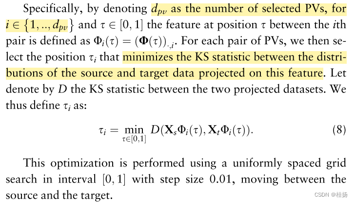
This process is important for every top $d_{pv}$ PVs It has to be repeated ,resulting in an optimal interpolation position for each. Then insert these positions back into geodesic curve, obtain domain-invariant feature representation $F$, Defined as ：

Notes on implementation

Once the number of principal components and PVs have been set (see Supplementary Subsection 5 for an example), the only hyper-parameter that needs to be optimized is the shrinkage coefficient (k) in the regression model. We employed a nested 10-fold cross-validation for this purpose. Specifically, for each of the outer cross-validation folds, we employed an inner 10-fold cross-validation on 90% of the data (the outer training fold) to estimate the optimal k.To this end, in each of the 10 inner folds, we estimated the common subspace, projected the inner training and test fold on the subspace, trained a predictor on the projected inner training fold and deter- mined the performance on the projected inner test fold as a function of k. After completing these steps for all 10 inner folds, we determined the optimal k across these results. Then we trained a model with the optimal k on the outer training fold and applied the predictor to the remaining 10% of the data (outer test fold). We then employed the Pearson correlation between the predicted and actual values on the outer test folds as a metric of predictive performance. Note that every sample in an outer test folds is never employed to perform either domain adaptation nor in constructing the response predictor in that same fold.

The methodology presented in this section is available as a Python 3.7 package available on our GitHub page. The domain adaptation step has been fully coded by ourselves and the regression and cross-validation uses scikit-learn 0.19.2 (Pedregosa et al., 2011).