Opencv image processing - grayscale processing

1、 linear transformation

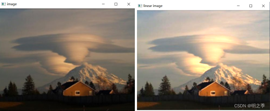
• The linear transformation of gray scale will press the values of all pixels in the image Linear transformation function To transform .
• In the case of underexposure or overexposure , The gray value of the image will be limited to a very small range , What you see on the monitor is a blur 、 There seems to be no hierarchy of images .
• In this case , A linear single value function is used to linearly extend each pixel in the image , Will effectively Improve the visual effect of the image .
• The principle of linear transformation is shown in the figure .
  
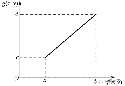
  According to the picture above , Take underexposure for example , Suppose the original image f(x,y) The gray scale range of is [a,b], The image expected to be obtained after linear transformation of gray level g(x,y) The gray scale range is [c,d], Then the linear transformation process is as follows .
  
  A more general mathematical expression is ：
  
  among ,g(x, y) Is the transformed value ,a Is the coefficient ,b Constant term .

# 1、 linear transformation 
import cv2
import numpy as np

img = cv2.imread('img.jpg')
cv2.imshow('image', img)
# cv2.waitKey(0)
#  linear transformation 
linear_img = 1.5 * img + 10
linear_img.max()    #  Maximum 364.0
#  truncation , The greater than 255 The pixel value of becomes 255
linear_img[linear_img>255] = 255
linear_img = np.asarray(linear_img, np.uint8) #  The pixel value becomes an integer 
cv2.imshow('linear image', linear_img)
cv2.waitKey(0)

2、 Nonlinear transformation

• Use non-linear function to map image gray , It can realize the nonlinear transformation of image gray , Commonly used logarithmic functions and exponential functions are typical logarithmic functions （ chart （a））、 Exponential function （ chart （b）） etc. .
  

2.1 Logarithmic transformation

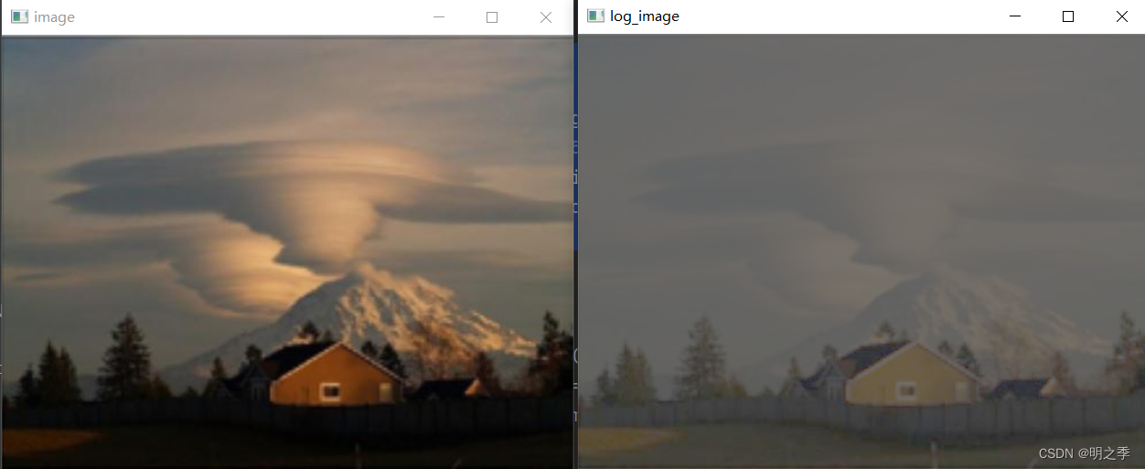
• Logarithmic transformation You can enhance pixels with low gray values , Expand the low gray area , Suppress pixels with high gray values , When you want to stretch the low gray area of an image and compress the high gray area , This transformation can be used .
• Because the logarithmic curve has a large slope in areas with low pixel values , In the area with higher pixel value, the slope is smaller , So the image is transformed by logarithm , The contrast of darker areas will be improved . Can be used for Enhance the dark details of the image , Thus, it is used to expand the darker pixels in the compressed high-value image .
  
  

# 2.  Nonlinear transformation 
#  Logarithmic transformation 
log_img = 10 + 20 * np.log(img+5)
#  truncation , The greater than 255 The pixel value of becomes 255
log_img[log_img>255] = 255    
log_img = np.asarray(log_img, np.uint8) #  The pixel value becomes an integer 
cv2.imshow('log_image', log_img)
cv2.imshow('image', img)
cv2.waitKey(0)

2.2 Exponential transformation

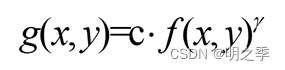
• Exponential transformation （ Gamma transform ） It is used for image enhancement , Improve dark details , In short, it is a nonlinear transformation , Let the image change from the linear response of exposure intensity to the response of human eyes , namely Will bleach （ Camera exposure ） Or too dark （ Underexposure ） Pictures of the , To correct .
• The expression of exponential transformation is shown in the formula .
  
  
  

#  Exponential transformation 
gamma_img = 10 * np.power(img, 1.1)
#  truncation , The greater than 255 The pixel value of becomes 255
gamma_img[gamma_img>255] = 255    
#  The pixel value becomes an integer 
gamma_img = np.asarray(gamma_img, np.uint8) 
cv2.imshow('gamma_image', gamma_img)
cv2.imshow('image', img)
cv2.waitKey(0)

3、 Histogram Processing

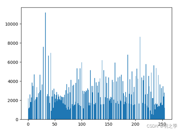
• The gray histogram of the image is shown in the figure , Use abscissa to represent gray level , The ordinate represents the number of pixels in each gray level .
• Through the gray histogram can reflect the statistical characteristics of image gray , And the proportion of the area or the number of pixels with different gray values in the whole image .
  
• In the two gray-scale histograms shown in the figure , If histogram is densely distributed in a very narrow area , It means that the contrast of the image is very low ; If histogram has two peaks , It indicates that there may be two areas with different brightness in the image .
  
• Histogram is one-dimensional feature of image , An image has a unique histogram . The distribution of gray level of image histogram can provide many features of image information , Provide a powerful argument for image analysis .
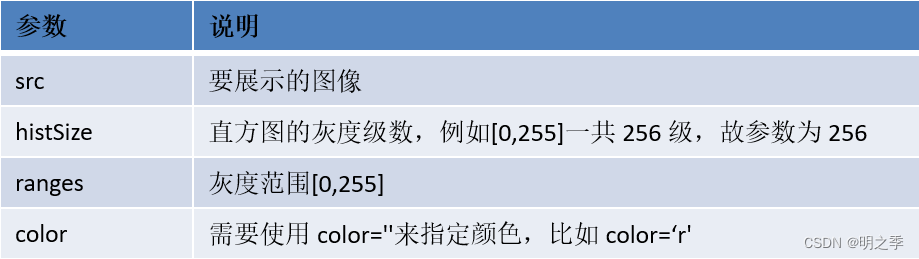
• View the histogram distribution of the image ： plt.hist(src.ravel(),hitsizes, ranges, color)
  

import cv2
import numpy as np
import matplotlib.pyplot as plt

#  Gray histogram of the image 
img = cv2.imread('img.jpg')
#  Draw a gray histogram 
plt.hist(img.ravel(), 256, [0,255])

3.1 Histogram equalization

• The basic idea of histogram equalization is to do some mapping transformation on the gray level of pixels in the original image , The probability density of the gray level of the transformed image is uniformly distributed , That is, the transformed image is an image with uniform gray level distribution , This means that the dynamic range of image gray is increased , thus Improve the contrast of the image .
• To achieve histogram equalization, you can use ：cv2.equalizeHist(src),
  src Single channel image is required .
  Histogram equalization of gray image is as follows ：
  

#  Histogram equalization 
img_gray = cv2.cvtColor(img, cv2.COLOR_BGR2GRAY)    #  Turn to grayscale 
img_hist = cv2.equalizeHist(img_gray)   #  Equalize the single channel image 
cv2.imshow('gray', img_gray)
cv2.imshow('hist', img_hist)
cv2.waitKey(0)

3.2 Histogram equalization of color image

• To perform histogram equalization on multi-channel images , First, separate the channels of the original image , Then histogram equalization is carried out respectively , Finally, the processed single channel images can be merged .
• Channel segmentation can be done by cv2.split() Realization , such as ：b, g, r = cv2.split(img)
• Channel merging is similar to array merging , adopt cv2.merge() Realization , such as ：cv2.merge((bH, gH, rH))
  
  

#  Histogram equalization of color image 
def EqualizeHist(img):
    # 1.  Split channels 
    (b, g, r) = cv2.split(img)
    # 2.  Equalize each channel separately 
    bh = cv2.equalizeHist(b)
    gh = cv2.equalizeHist(g)
    rh = cv2.equalizeHist(r)
    # 3.  Merge 
    result = cv2.merge((bh, gh, rh))
    return result

#  Histogram equalization of the original image 
img_equal = EqualizeHist(img)
cv2.imshow('image', img)
cv2.imshow('image_equal', img_equal)
cv2.waitKey(0)
#  Draw histogram 
plt.hist(img_equal.ravel(), 256, [0,255])

4、 Two valued

• Binarization is the value that keeps the image black and white , Black and white .
  • Color images ： Three channels , Pixel values 0-255,0-255,0-255, So you can have 2^24 Bitspace
  • Grayscale image ： A passage , Pixel values 0-255, So there is 256 Color
  • Binary image ： Only two colors , Black and white ,255 white ,0 black
• Image binarization （Image Binarization） Is to set the gray value of pixels on the image to 0 or 255, That is to say, the process of presenting the whole image with obvious black-and-white effect .
• In digital image processing , Binary image plays a very important role , The binarization of the image greatly reduces the amount of data in the image , So as to highlight the outline of the target .
• OpenCV There are two ways to realize the binarization of images ：
  • Threshold truncation ： Select a global threshold , With this value as the boundary, the whole image is divided into binary images that are either black or white .
  • cv2.threshold(src, thresh, maxval, type)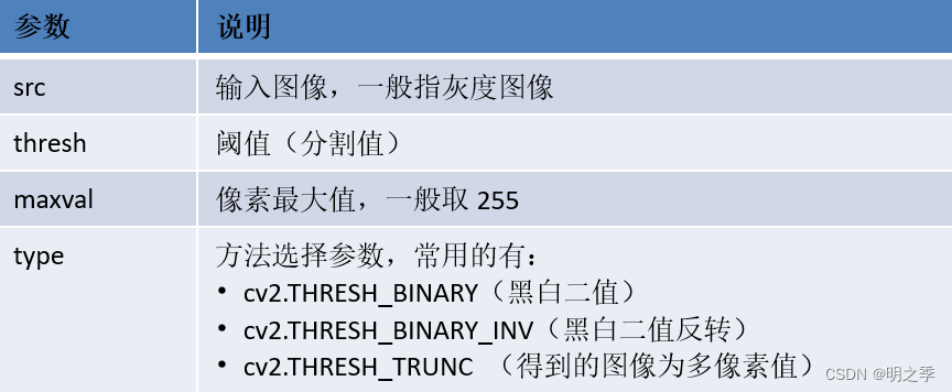
  

#  Two valued 
# 1.  Threshold truncation 
img = cv2.imread('img.jpg')
img_gray = cv2.cvtColor(img, cv2.COLOR_BGR2GRAY)
_, img_binary = cv2.threshold(src=img_gray, thresh=50, maxval=255,
                         type=cv2.THRESH_BINARY)
cv2.imshow('image_binary', img_binary)
cv2.imshow('image', img)
cv2.waitKey(0)

• OpenCV There are two ways to realize the binarization of images ：
  • Adaptive threshold ： Adaptive threshold can be regarded as a kind of local threshold , By specifying the size of an area , Compare this point with the average value of pixels in the area size （ Or other characteristics ） The size relationship determines whether the pixel belongs to black or white .
  • cv2.adaptiveThreshold(src, maxValue, adaptiveMethod, thresholdType, blockSize, C)
  

# 2. Adaptive threshold 
adapt_thres = cv2.adaptiveThreshold(src=img_gray, maxValue=255,
                              adaptiveMethod=cv2.ADAPTIVE_THRESH_GAUSSIAN_C,
                              thresholdType=cv2.THRESH_BINARY,
                              blockSize=9, C=3)
cv2.imshow('adapt image', adapt_thres)
cv2.waitKey(0)