当前位置:网站首页>随机森林项目实战---气温预测
随机森林项目实战---气温预测
2022-08-03 12:02:00 【羊咩咩咩咩咩】
实战项目的三个任务:
1.使用随机森林算法完成基本建模:包括数据预处理,特征展示,完成建模并进行可视化展示分析。
2.分析数据样本量与特征个数对结果的影响,在保证算法一致的前提下,增加样本个数,观察结果变化,重新进行特征工程,引入新的特征后,观察结果走势。
3.对随机森林算法进行调参,找到最合适的参数,掌握机器学习中两种调参方法,找到模型最优参数。
任务1:
import pandas as pd
data =pd.read_csv()
data.head()
import datetime
year = data['year']
month  =data['month']
day =data['day']
dates = [(str(year)+'-'+str(month)+'-'+str(day)) for year,month,day in  zip(year,month,day)]
dates=[datetime.datetime.strptime(date,'%Y-%m-%d') for date in dates]
dates[:5]
对时间序列进行重新调整,进行特征绘制。
##进行绘图
import matplotlib.pyplot as plt
%matplotlib inline
plt.style.use('fivethirtyeight')##风格设置
# 设置布局
fig, ((ax1, ax2), (ax3, ax4)) = plt.subplots(nrows=2, ncols=2, figsize = (10,10))
fig.autofmt_xdate(rotation = 45)

# 标签值
ax1.plot(dates, data['actual'])
ax1.set_xlabel(''); ax1.set_ylabel('Temperature'); ax1.set_title('Max Temp')

# 昨天
ax2.plot(dates, data['temp_1'])
ax2.set_xlabel(''); ax2.set_ylabel('Temperature'); ax2.set_title('Previous Max Temp')

# 前天
ax3.plot(dates, data['temp_2'])
ax3.set_xlabel('Date'); ax3.set_ylabel('Temperature'); ax3.set_title('Two Days Prior Max Temp')

# 我的逗逼朋友
ax4.plot(dates, data['friend'])
ax4.set_xlabel('Date'); ax4.set_ylabel('Temperature'); ax4.set_title('Friend Estimate')

plt.tight_layout(pad=2)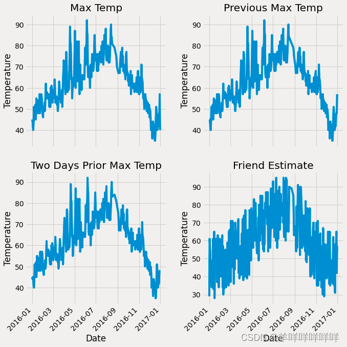
从中可以看出4个特征的基本影响走势。
import numpy as np
y = np.array(data['actual'])
x = data.drop(['actual'],axis=1)
x_list =list(x.columns)
x = np.array(x)
##数据分类
from sklearn.model_selection import train_test_split
x_train,x_test,y_train,y_test =train_test_split(x,y,test_size=0.25,random_state=42)
##建立随机森林模型
from sklearn.ensemble import RandomForestRegressor
rfr = RandomForestRegressor(n_estimators=1000,random_state=42)
rfr.fit(x_train,y_train)
y_pred = rfr.predict(x_test)
from sklearn.metrics import mean_squared_error
mse=mean_squared_error(y_test,y_pred)
print('mse',mse)
这里进行了测试集与训练集的分割与随机森林模型的建立。通过建立的模型预测了结果与真实值计算量mse的值。
随后进行了决策树树的可视化
from sklearn.tree import export_graphviz
import pydot
tree = rfr.estimators_[5]
export_graphviz(tree,out_file='tree.dot',
               feature_names=x_list,
               rounded=True,precision=1)
(graph,) = pydot.graph_from_dot_file('tree.dot')
graph.write_png('tree.png')
由于树枝过于复杂繁多,所以进行预剪枝。
##进行预剪枝
rfr_small = RandomForestRegressor(n_estimators=10,max_depth=3,random_state=42)
rfr_small.fit(x_train,y_train)
tree_small = rfr_small.estimators_[5]
export_graphviz(tree_small,out_file='small_tree.dot',
               feature_names=x_list,
               rounded=True,precision=1)
(graph,) = pydot.graph_from_dot_file('small_tree.dot')
graph.write_png('small_tree.png')
2.选择出重点的特征,然后对全特征与重点特征的结果进行比较
这里使用了randomforestregressor.feature_importance_可以输出重要值。
##通过randomforestregressor的feature_importance_显示特征重要性
importance = list(rfr.feature_importances_)
feature_importances =[(feature_name,importance) for feature_name,importance in zip(x_list,importance)]
feature_importances =sorted(feature_importances,key =lambda x:x[1],reverse =True)##key 为以那一列数据为排列对象
feature_importances
##以这两个特征为唯二的特征进行计算
rfr = RandomForestRegressor(n_estimators=100,random_state=42)
new_x = np.array(data.iloc[:,4:5])
new_x_train,new_x_test,new_y_train,new_y_test =train_test_split(new_x,y,test_size=.25,random_state=42)
rfr.fit(new_x_train,new_y_train)
y_pred = rfr.predict(new_x_test)
print('mse',mean_squared_error(new_y_test,y_pred))
相比之下,mse值上升,说明效果不好,其他特征有也重要效果。
任务二:数据与特征对结果的影响分析。
这里读取了数据的拓展包进行测试。操作与上面的一样
import pandas as pd
data =pd.read_csv()
data.head()
##绘图观察数据
# 转换成标准格式
import datetime

# 得到各种日期数据
years = data['year']
months = data['month']
days = data['day']

# 格式转换
dates = [str(int(year)) + '-' + str(int(month)) + '-' + str(int(day)) for year, month, day in zip(years, months, days)]
dates = [datetime.datetime.strptime(date, '%Y-%m-%d') for date in dates]

# 绘图
import matplotlib.pyplot as plt

%matplotlib inline

# 风格设置
plt.style.use('fivethirtyeight')
# Set up the plotting layout
fig, ((ax1, ax2), (ax3, ax4)) = plt.subplots(nrows=2, ncols=2, figsize = (15,10))
fig.autofmt_xdate(rotation = 45)

# Actual max temperature measurement
ax1.plot(dates, data['actual'])
ax1.set_xlabel(''); ax1.set_ylabel('Temperature (F)'); ax1.set_title('Max Temp')

# Temperature from 1 day ago
ax2.plot(dates, data['temp_1'])
ax2.set_xlabel(''); ax2.set_ylabel('Temperature (F)'); ax2.set_title('Prior Max Temp')

# Temperature from 2 days ago
ax3.plot(dates, data['temp_2'])
ax3.set_xlabel('Date'); ax3.set_ylabel('Temperature (F)'); ax3.set_title('Two Days Prior Max Temp')

# Friend Estimate
ax4.plot(dates, data['friend'])
ax4.set_xlabel('Date'); ax4.set_ylabel('Temperature (F)'); ax4.set_title('Friend Estimate')

plt.tight_layout(pad=2)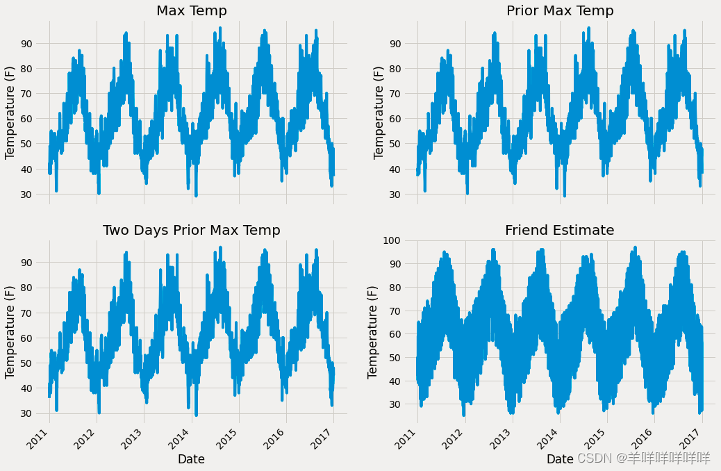
由于多了特征,对多出来的特征进行组合与处理。
seasons=[]
for month in data['month']:
    if month in[1,2,12]:
        seasons.append('winter')
    elif month in [3,4,5]:
        seasons.append('spring')
    elif month in [6,7,8]:
        seasons.append('summer')
    else:
        seasons.append('auntumn')
reduced_x = data[['temp_1','prcp_1','average','actual']]
reduced_x['seasons']=seasons
# 导入seaborn工具包
import seaborn as sns
sns.set(style="ticks", color_codes=True);

# 选择你喜欢的颜色模板
palette = sns.xkcd_palette(['dark blue', 'dark green', 'gold', 'orange'])

# 绘制pairplot
sns.pairplot(reduced_x, hue = 'seasons', diag_kind = 'kde', palette= palette, plot_kws=dict(alpha = 0.7),
diag_kws=dict(shade=True)); 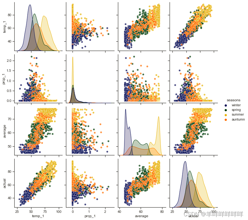
画出了四个月气温变化的相关图。
先改变数据量,测试数据量对模型效果的影响。
data = pd.get_dummies(data)
new_y = np.array(data['actual'])
new_x = data.drop(['actual'],axis=1)
new_x_list =list(new_x.columns)
new_x = np.array(new_x)
from sklearn.model_selection import train_test_split
new_x_train,new_x_test,new_y_train,new_y_test =train_test_split(new_x,new_y,test_size=0.25,random_state=42)
old_y = np.array(data['actual'])
old_x = data.drop(['actual'],axis=1)
old_x_list =list(old_x.columns)
old_x = np.array(old_x)
from sklearn.model_selection import train_test_split
old_x_train,old_x_test,old_y_train,old_y_test =train_test_split(x,y,test_size=0.25,random_state=42)
def model_train_predict(x_train,y_train,x_test,y_test):
    rfr = RandomForestRegressor(n_estimators=100,random_state=42)
    rfr.fit(x_train,y_train)
    y_pred = rfr.predict(x_test)
    errors= abs(y_pred-y_test)
    print('平均误差',round(np.mean(errors),2))
    accuracy = 100-np.mean(errors)
    print('平均正确率',accuracy)
model_train_predict(old_x_train,old_y_train,old_x_test,old_y_test)
model_train_predict(ori_new_x_train,new_y_train,ori_new_x_test,new_y_test)
从结果可以发现,当数据量增加,误差减少。
然后改变特征数量,判断其对效果的影响。
rfr = RandomForestRegressor(n_estimators=100,random_state=42)
rfr.fit(new_x_train,new_y_train)
y_pred = rfr.predict(new_x_test)
errors= abs(y_pred-new_y_test)
print('平均误差',round(np.mean(errors),2))
accuracy = 100-np.mean(errors)
print('平均正确率',accuracy)
importances = list(rfr.feature_importances_)
feature_importances  =[(feature,importance) for feature,importance in zip(new_x_list,importances)]
feature_importances = sorted(feature_importances,key =lambda x:x[1],reverse =True)
# 对特征进行排序
x_values =list(range(len(importances)))
sorted_importances = [importance[1] for importance in feature_importances]
sorted_features = [importance[0] for importance in feature_importances]

# 累计重要性
cumulative_importances = np.cumsum(sorted_importances)

# 绘制折线图
plt.plot(x_values, cumulative_importances, 'g-')

# 画一条红色虚线,0.95那
plt.hlines(y = 0.95, xmin=0, xmax=len(sorted_importances), color = 'r', linestyles = 'dashed')

# X轴
plt.xticks(x_values, sorted_features, rotation = 'vertical')

# Y轴和名字
plt.xlabel('Variable'); plt.ylabel('Cumulative Importance'); plt.title('Cumulative Importances');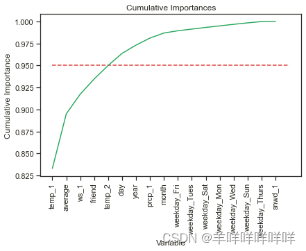
根据主成分分析,总重要性大于95%基本可以概括为这5个特征可以涵盖所有重要性。
important_feature_names =[feature[0] for feature in feature_importances[0:5]]
important_feature_indices =[new_x_list.index(feature) for feature in important_feature_names]
important_x_train = new_x_train[:,important_feature_indices]
important_x_test = new_x_test[:,important_feature_indices]
model_train_predict(important_x_train,new_y_train,important_x_test,new_y_test)
##运行时间的提升
import time
all_features_time=[]
for _ in range(10):
    start_time = time.time()
    rfr.fit(new_x_train,new_y_train)
    y_pred = rfr.predict(new_x_test)
    end_time =time.time()
    all_features_time.append((end_time-start_time))
all_features_times=np.mean(all_features_time)
all_features_time=[]
for _ in range(10):
    start_time = time.time()
    rfr.fit(important_x_train,new_y_train)
    y_pred = rfr.predict(important_x_test)
    end_time =time.time()
    all_features_time.append((end_time-start_time))
reduced_features_times=np.mean(all_features_time)
all_accuracy =100*(1-np.mean(abs(all_y_pred-new_y_test)/new_y_test))
reduced_accuracy =100*(1-np.mean(abs(reduced_y_pred-new_y_test)/new_y_test))
comparison = pd.DataFrame({'features': ['all (17)', 'reduced (5)'],
                           'run_time': [all_features_times, reduced_features_times],
                           'accuracy': [all_accuracy, reduced_accuracy]})

comparison[['features', 'accuracy', 'run_time']]
这里通过比较对运行时间的优化与正确率的提升进行比较,发现当数据量多与特征多的时候,对模型建立的效果越好。
任务三:调参:这里使用RandomizeSearchCV与GridSearchCV两种调参方式进行参数的选择。
from sklearn.model_selection import RandomizedSearchCV
n_estimators =[int(x) for x in np.linspace(start=200,stop=2000,num=10)]
max_features=['auto','sqrt']
max_depth = [int(x) for x in np.linspace(10,20,num=2)]
max_depth.append(None)
min_samples_split=[2,5,10]
min_samples_leaf=[1,2,4]
bootstrap = [True,False]
random_grid = {'n_estimators': n_estimators,
               'max_features': max_features,
               'max_depth': max_depth,
               'min_samples_split': min_samples_split,
               'min_samples_leaf': min_samples_leaf,
               'bootstrap': bootstrap}
rf = RandomForestRegressor()

rf_random = RandomizedSearchCV(estimator=rf, param_distributions=random_grid,
                              n_iter = 100, scoring='neg_mean_absolute_error',
                              cv = 3, verbose=2, random_state=42, n_jobs=-1)

# 执行寻找操作
rf_random.fit(new_x_train, new_y_train)
from sklearn.model_selection import GridSearchCV

# 网络搜索
param_grid = {
    'bootstrap': [True],
    'max_depth': [8,10,12],
    'max_features': ['auto'],
    'min_samples_leaf': [2,3, 4, 5,6],
    'min_samples_split': [3, 5, 7],
    'n_estimators': [800, 900, 1000, 1200]
}

# 选择基本算法模型
rf = RandomForestRegressor()

# 网络搜索
grid_search = GridSearchCV(estimator = rf, param_grid = param_grid,
                           scoring = 'neg_mean_absolute_error', cv = 3,
                           n_jobs = -1, verbose = 2)
grid_search.fit(train_features, train_labels)
最后发现可以通过随机搜索确定大方向,使用网格化搜索进行精细化搜索
边栏推荐
猜你喜欢
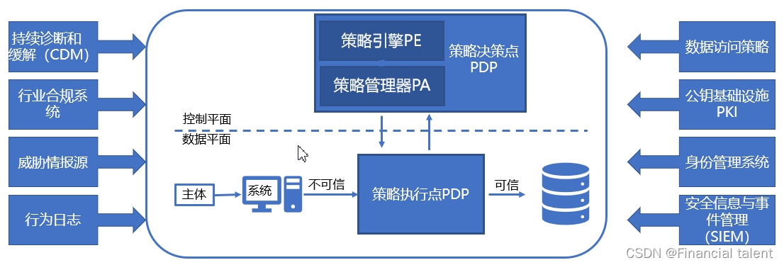
零信任架构分析【扬帆】
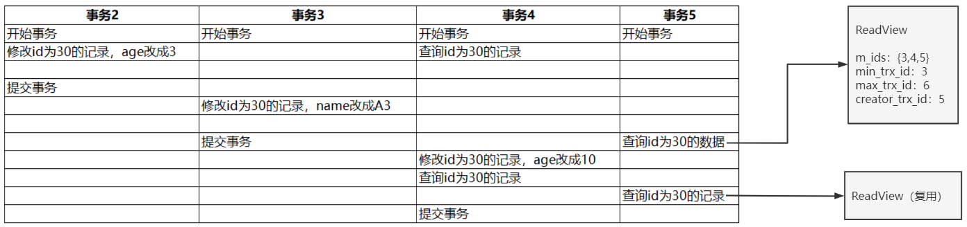
深入理解MySQL事务MVCC的核心概念以及底层原理
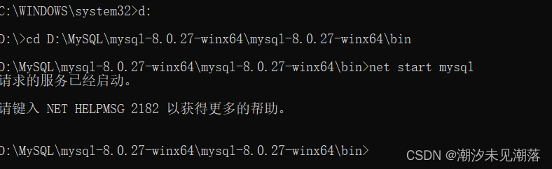
net start mysql 启动报错:发生系统错误5。拒绝访问。
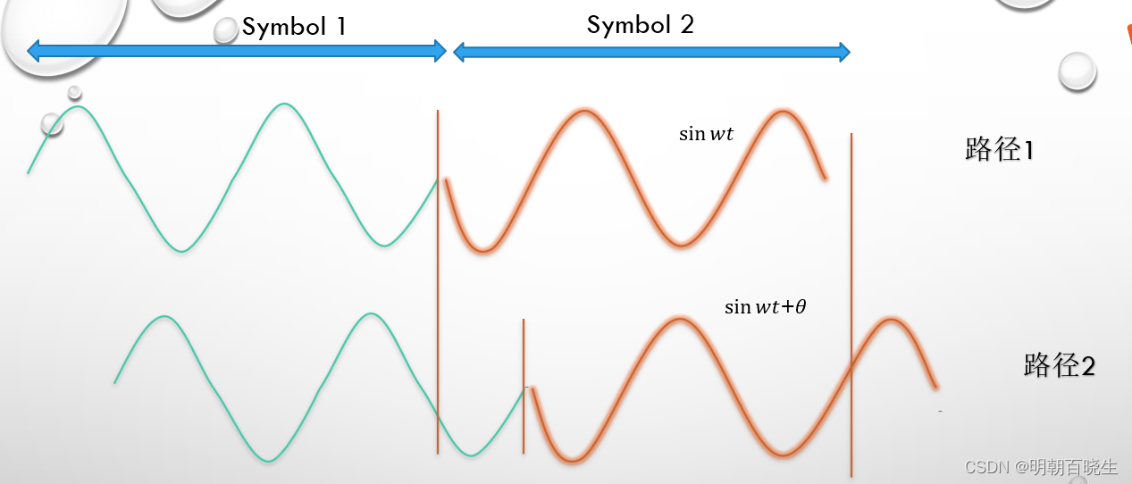
OFDM 十六讲 4 -What is a Cyclic Prefix in OFDM
![LeetCode 899 Ordered queue [lexicographical order] HERODING's LeetCode road](/img/95/1b63cfb25b9e0802666114f089fcb8.png)
LeetCode 899 Ordered queue [lexicographical order] HERODING's LeetCode road

分享一款实用的太阳能充电电路(室内光照可用)

fastposter v2.9.0 programmer must-have poster generator

word标尺有哪些作用

Redis发布订阅和数据类型
从零开始C语言精讲篇5:指针
随机推荐
【一起学Rust 基础篇】Rust基础——变量和数据类型
bash case usage
为什么越来越多的开发者放弃使用Postman,而选择Eolink?
微信小程序获取手机号
dataset数据集有哪些_数据集类型
从零开始C语言精讲篇5:指针
距LiveVideoStackCon 2022 上海站开幕还有3天!
苹果发布 AI 生成模型 GAUDI,文字生成 3D 场景
pandas连接oracle数据库并拉取表中数据到dataframe中、生成当前时间的时间戳数据、格式化为指定的格式(“%Y-%m-%d-%H-%M-%S“)并添加到csv文件名称中
矩阵的计算[通俗易懂]
opencv学习—VideoCapture 类基础知识「建议收藏」
R语言绘制时间序列的自相关函数图:使用acf函数可视化时间序列数据的自相关系数图
永寿 永寿农特产品-苹果
PC client automation testing practice based on Sikuli GUI image recognition framework
码率vs.分辨率,哪一个更重要?
LyScript implements memory stack scanning
"Digital Economy Panorama White Paper" Financial Digital User Chapter released!
LeetCode-1796. 字符串中第二大的数字
[论文阅读] (23)恶意代码作者溯源(去匿名化)经典论文阅读:二进制和源代码对比
Vs 快捷键---探索不一样的编程