Time series forecasting based on trend and seasonality

Time series forecasting is the task of forecasting based on time data . It involves building models to make observations , And in places like weather 、 engineering 、 economic 、 Applications such as financial or business forecasting drive future decisions .

This paper mainly introduces time series prediction and describes the two main models of any time series ( Trends and seasonality ). Based on these patterns, the time series are decomposed . The last one is called Holt-Winters Prediction model of seasonal method , To predict trends and / Or time series data of seasonal components .

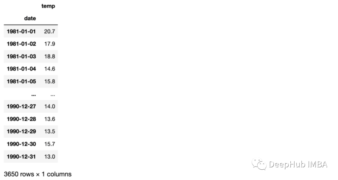
To cover all this , We will use a time series data set , Include 1981 - 1991 Melbourne during the year ( Australia ) Temperature of . This data set can be obtained from this Kaggle download , You can also use the last part of this article GitHub download , It contains the data and code of this article . This data set is hosted by the Australian government meteorological service , And according to the “ Default terms of use ”(Open Access Licence) Get permission to .

Import libraries and data

First , Import the following libraries needed to run the code . In addition to the most typical Libraries , The code is also based on statsmomodels Functions provided by the library , The library provides classes and functions for estimating many different statistical models , Such as statistical test and prediction model .

from datetime import datetime, timedelta
import matplotlib.pyplot as plt
import numpy as np
import pandas as pd
import statsmodels.api as sm
from statsmodels.tsa.stattools import adfuller, kpss
from statsmodels.tsa.api import ExponentialSmoothing
%matplotlib inline

Here is the code for importing data . The data consists of two columns , One column is the date , The other column is 1981 - 1991 Melbourne in ( Australia ) Temperature of .

# date
numdays = 365*10 + 2
base = '2010-01-01'
base = datetime.strptime(base, '%Y-%m-%d')
date_list = [base + timedelta(days=x) for x in range(numdays)]
date_list = np.array(date_list)
print(len(date_list), date_list[0], date_list[-1])

# temp
x = np.linspace(-np.pi, np.pi, 365)
temp_year = (np.sin(x) + 1.0) * 15
x = np.linspace(-np.pi, np.pi, 366)
temp_leap_year = (np.sin(x) + 1.0)
temp_s = []
for i in range(2010, 2020):
    if i == 2010:
        temp_s = temp_year + np.random.rand(365) * 20
    elif i in [2012, 2016]:
        temp_s = np.concatenate((temp_s, temp_leap_year * 15 + np.random.rand(366) * 20 + i % 2010))
    else:
        temp_s = np.concatenate((temp_s, temp_year + np.random.rand(365) * 20 + i % 2010))
print(len(temp_s))

# df
data = np.concatenate((date_list.reshape(-1, 1), temp_s.reshape(-1, 1)), axis=1)
df_orig = pd.DataFrame(data, columns=['date', 'temp'])
df_orig['date'] =  pd.to_datetime(df_orig['date'], format='%Y-%m-%d')
df = df_orig.set_index('date')
df.sort_index(inplace=True)
df

Visual datasets

Before we start analyzing the patterns of time series , Let's visualize each vertical dotted line corresponding to the data at the beginning of the year .

ax = df_orig.plot(x='date', y='temp', figsize=(12,6))
xcoords = ['2010-01-01', '2011-01-01', '2012-01-01', '2013-01-01', '2014-01-01',
           '2015-01-01', '2016-01-01', '2017-01-01', '2018-01-01', '2019-01-01']
for xc in xcoords:
    plt.axvline(x=xc, color='black', linestyle='--')
ax.set_ylabel('temperature')

Before moving on to the next section , Let's take a moment to look at the data . These data seem to have a seasonal variation , The temperature rises in winter , The temperature drops in summer ( southern hemisphere ). And the temperature doesn't seem to increase with time , Because the average temperature is the same in any year .

Time series patterns

The time series prediction model uses mathematical equations (s) Find patterns in a series of historical data . Then use these equations to put the data [ The historical time pattern in is projected into the future .

There are four types of time series patterns :

trend : Long term increase and decrease of data . A trend can be any function , Such as linear or exponential , And can change direction over time .

Seasonality : At a fixed frequency ( Hours of the day 、 week 、 month 、 Years etc. ) A cycle repeated in a series . The seasonal pattern has a fixed known period

periodic : Occurs when the data goes up or down , But there is no fixed frequency and duration , For example, caused by economic conditions .

The noise : Random variations in the series .

Most time series data will contain one or more patterns , But maybe not all . Here are some examples , We can identify these time series patterns :

Wikipedia's audience of the year ( On the left ): In this picture , We can identify an increasing trend , The audience increases linearly every year .

Us electricity consumption seasonal chart ( Chinese ): Each line corresponds to a year , Therefore, we can observe the seasonality of repeated electricity consumption every year .

ibex35 Daily closing price of ( Right picture ): This time series has an increasing trend with the passage of time , And a periodic pattern , Because there are some periods ibex35 Decline due to economic reasons .

If we assume that these patterns are additive decomposed , We can write this way :

Y[t] = t [t] + S[t] + e[t]

among Y[t] For data ,t [t] Is the trend period component ,S[t] Is the seasonal component ,e[t] Is noise ,t Is the time period .

On the other hand , Multiplicative decomposition can be written as :

Y[t] = t [t] *S[t] *e[t]

When the seasonal fluctuation does not change with the time series level , Additive decomposition is the most appropriate method . contrary , When the change of seasonal components is proportional to the level of time series , It is more suitable to use multiplication decomposition .

Decomposing data

A stationary time series is defined as one that is independent of the time at which it is observed . Therefore, time series with trend or seasonality are not stable , The white noise sequence is stationary . Mathematically speaking , If the mean and variance of a time series do not change , And the covariance is independent of time , So this time series is stationary . There are different examples to compare stationary and nonstationary time series . Generally speaking , Stationary time series do not have long-term predictable patterns .

Why is stability important ?

Stationarity has become a common assumption of many practices and tools in time series analysis . This includes trend estimation 、 Prediction and causal inference . therefore , in many instances , It is necessary to determine whether the data is generated by a fixed process , And convert it into an attribute with the sample generated by the process .

How to test the stationarity of time series ?

We can test it in two ways . One side , We can check manually by checking the mean and variance of the time series . On the other hand , We can use test functions to evaluate stationarity .

Some situations can be confusing . For example, a time series without trend and seasonality but with periodic behavior is stable , Because the length of the period is not fixed .

Check the trend

In order to analyze the trend of time series , We first use the 30 The rolling mean method of the day window is used to analyze the mean value over time .

def analyze_stationarity(timeseries, title):
    fig, ax = plt.subplots(2, 1, figsize=(16, 8))

    rolmean = pd.Series(timeseries).rolling(window=30).mean() 
    rolstd = pd.Series(timeseries).rolling(window=30).std()
    ax[0].plot(timeseries, label= title)
    ax[0].plot(rolmean, label='rolling mean');
    ax[0].plot(rolstd, label='rolling std (x10)');
    ax[0].set_title('30-day window')
    ax[0].legend()
    
    rolmean = pd.Series(timeseries).rolling(window=365).mean() 
    rolstd = pd.Series(timeseries).rolling(window=365).std()
    ax[1].plot(timeseries, label= title)
    ax[1].plot(rolmean, label='rolling mean');
    ax[1].plot(rolstd, label='rolling std (x10)');
    ax[1].set_title('365-day window')
    
pd.options.display.float_format = '{:.8f}'.format
analyze_stationarity(df['temp'], 'raw data')
    ax[1].legend()

In the diagram above , We can see the use of 30 How the rolling mean of the day window fluctuates with time , This is caused by the seasonal pattern of the data . Besides , When using 365 Day window , The rolling average increases over time , Indicates a slight increase over time .

This can also be evaluated by some tests , Such as Dickey-Fuller (ADF) and Kwiatkowski, Phillips, Schmidt and Shin (KPSS):

ADF The results of the test (p The value is less than 0.05) indicate , The original assumption of existence can be made in 95% Rejected at the confidence level of . therefore , If p The value is less than 0.05, Then the time series is stable .

def ADF_test(timeseries):
    print("Results of Dickey-Fuller Test:")
    dftest = adfuller(timeseries, autolag="AIC")
    dfoutput = pd.Series(
        dftest[0:4],
        index=[
            "Test Statistic",
            "p-value",
            "Lags Used",
            "Number of Observations Used",
        ],
    )
    for key, value in dftest[4].items():
        dfoutput["Critical Value (%s)" % key] = value
    print(dfoutput)

ADF_test(df)

Results of Dickey-Fuller Test:
Test Statistic                  -3.69171446
p-value                          0.00423122
Lags Used                       30.00000000
Number of Observations Used   3621.00000000
Critical Value (1%)             -3.43215722
Critical Value (5%)             -2.86233853
Critical Value (10%)            -2.56719507
dtype: float64

KPSS The results of the test (p The value is higher than 0.05) indicate , stay 95% At a confidence level of , The irresistible null hypothesis . So if p The value is less than 0.05, Then the time series is not stable .

def KPSS_test(timeseries):
    print("Results of KPSS Test:")
    kpsstest = kpss(timeseries.dropna(), regression="c", nlags="auto")    
    kpss_output = pd.Series(
        kpsstest[0:3], index=["Test Statistic", "p-value", "Lags Used"]
    )
    for key, value in kpsstest[3].items():
        kpss_output["Critical Value (%s)" % key] = value
    print(kpss_output)

KPSS_test(df)

Results of KPSS Test:
Test Statistic           1.04843270
p-value                  0.01000000
Lags Used               37.00000000
Critical Value (10%)     0.34700000
Critical Value (5%)      0.46300000
Critical Value (2.5%)    0.57400000
Critical Value (1%)      0.73900000
dtype: float64

Although these tests seem to check the stationarity of the data , But these tests are useful for analyzing the trend of time series rather than seasonality .

The statistical results also show the influence of the stationarity of time series . Although the null hypothesis of the two tests is opposite .ADF The test shows that the time series is stable (p value > 0.05), and KPSS The test shows that the time series is not stable (p value > 0.05). But this dataset was created with a slight trend , So the results show that ,KPSS Tests are more accurate for analyzing this data set .

In order to reduce the trend of the data set , We can use the following methods to eliminate trends :

df_detrend = (df - df.rolling(window=365).mean()) / df.rolling(window=365).std()

analyze_stationarity(df_detrend['temp'].dropna(), 'detrended data')
ADF_test(df_detrend.dropna())

Check seasonality

As observed from the sliding window before , There is a seasonal pattern in our time series . Therefore, the difference method should be used to remove the potential seasonal or periodic patterns in the time series . Because the sample data set has 12 Months of seasonality , I use the 365 Lag difference :

df_365lag =  df - df.shift(365)

analyze_stationarity(df_365lag['temp'].dropna(), '12 lag differenced data')
ADF_test(df_365lag.dropna())

Now? , The moving mean and standard deviation remain more or less constant over time , So we have a stationary time series .

The combined code of the above methods is as follows ：

df_365lag_detrend =  df_detrend - df_detrend.shift(365)

analyze_stationarity(df_365lag_detrend['temp'].dropna(), '12 lag differenced de-trended data')
ADF_test(df_365lag_detrend.dropna())

Decomposition mode

The decomposition based on the above schema can be achieved by ’ statmodels ' A useful in the package Python function seasonal_decomposition To achieve :

def seasonal_decompose (df):
    decomposition = sm.tsa.seasonal_decompose(df, model='additive', freq=365)

    trend = decomposition.trend
    seasonal = decomposition.seasonal
    residual = decomposition.resid

    fig = decomposition.plot()
    fig.set_size_inches(14, 7)
    plt.show()

    return trend, seasonal, residual

seasonal_decompose(df)

After looking at the four parts of the exploded view , so to speak , There is a strong seasonal component in our time series , And an increasing trend pattern over time .

Time series modeling

The appropriate model for time series data will depend on the specific characteristics of the data , for example , Does the data set have an overall trend or seasonality . Be sure to select the model that best fits the data .

We can use the following models ：

1. Autoregression (AR)
2. Moving Average (MA)
3. Autoregressive Moving Average (ARMA)
4. Autoregressive Integrated Moving Average (ARIMA)
5. Seasonal Autoregressive Integrated Moving-Average (SARIMA)
6. Seasonal Autoregressive Integrated Moving-Average with Exogenous Regressors (SARIMAX)
7. Vector Autoregression (VAR)
8. Vector Autoregression Moving-Average (VARMA)
9. Vector Autoregression Moving-Average with Exogenous Regressors (VARMAX)
10. Simple Exponential Smoothing (SES)
11. Holt Winter’s Exponential Smoothing (HWES)

Because of the seasonality in our data , So choose HWES, Because it applies to trends and / Or time series data of seasonal components .

This method uses exponential smoothing to encode a large number of past values , And use them to predict the present and future “ A typical ” value . Exponential smoothing refers to the use of exponential weighted moving average (EWMA)“ smooth ” A time series .

Before it's implemented , Let's create training and test data sets :

y = df['temp'].astype(float)
y_to_train = y[:'2017-12-31']
y_to_val = y['2018-01-01':]
predict_date = len(y) - len(y[:'2017-12-31'])

Here is the root mean square error (RMSE) Implementation as a measure to evaluate model errors .

def holt_win_sea(y, y_to_train, y_to_test, seasonal_period, predict_date):

    fit1 = ExponentialSmoothing(y_to_train, seasonal_periods=seasonal_period, trend='add', seasonal='add').fit(use_boxcox=True)
    fcast1 = fit1.forecast(predict_date).rename('Additive')
    mse1 = ((fcast1 - y_to_test.values) ** 2).mean()
    print('The Root Mean Squared Error of additive trend, additive seasonal of '+ 
          'period season_length={} and a Box-Cox transformation {}'.format(seasonal_period,round(np.sqrt(mse1), 2)))

    y.plot(marker='o', color='black', legend=True, figsize=(10, 5))
    fit1.fittedvalues.plot(style='--', color='red', label='train')
    fcast1.plot(style='--', color='green', label='test')
    plt.ylabel('temp')
    plt.title('Additive trend and seasonal')
    plt.legend()
    plt.show()

holt_win_sea(y, y_to_train, y_to_val, 365, predict_date)

The Root Mean Squared Error of additive trend, additive seasonal of period season_length=365 and a Box-Cox transformation 6.27

From the figure, we can see how the model captures the seasonality and trend of time series , There are some errors in the prediction of outliers .

summary

In this paper , We present trends and seasonality through a practical example based on temperature data sets . In addition to checking trends and seasonality , We also saw how to lower it , And how to create a basic model , Use these models to infer the temperature in the next few days .

It is very important to understand the main time series patterns and learn how to implement the time series prediction model , Because they have many applications .

This article data and code ：

https://avoid.overfit.cn/post/51c2316b0237445fbb3dbf6228ea3a52

author ：Javier Fernandez