当前位置:网站首页>Statistical analysis - data level description of descriptive statistics
Statistical analysis - data level description of descriptive statistics
2022-06-25 15:11:00 【A window full of stars and milky way】
Generally speaking, the numerical characteristics of a set of sample data can be described from three aspects :
Level of data ( It can also be called centralized trend or position measurement ), Reflecting data Value size
Differences in data , Reflect the... Between data The degree of dispersion
The distribution shape of the data , Reflecting the distribution of data skewness and kurtosis
Statistics describing the level
Data level refers to the size of the value , The statistics that describe the level of data are The average , quantile , The number of , At the same time, these statistics can also be used to describe the Concentration trend degree .
The average
** Simple average (simple mean)** Formula :
x ˉ = x 1 + x 2 + x 3 + . . . + x n n = ∑ i = 1 n x i n \bar{x} = \frac{x_{1}+x_{2}+x_{3}+...+x_{n}}{n} = \frac{\sum_{i=1}^{n}x_{i}}{n} xˉ=nx1+x2+x3+...+xn=n∑i=1nxi
Weighted average (weighted mean): If the sample is divided into K Group , Group median for each group ( The average of the upper and lower limits of the group ) by m1,m2,…,mk The frequency of each group is expressed in f1,f2,…,fk Express , Then the formula for calculating the average number of samples is :
x ˉ = m 1 f 1 + m 2 f 2 + m 3 f 3 + . . . + m k f k f 1 + f 2 + f 3 + . . . + f k = ∑ i = 1 k m i f i ∑ i = 1 k f i \bar{x} = \frac{m_{1}f_{1}+m_{2}f_{2}+m_{3}f_{3}+...+m_{k}f_{k}}{f_{1}+f_{2}+f_{3}+...+f_{k}} = \frac{\sum_{i=1}^{k}m_{i}f_{i}}{\sum_{i=1}^{k}f_{i}} xˉ=f1+f2+f3+...+fkm1f1+m2f2+m3f3+...+mkfk=∑i=1kfi∑i=1kmifi
Generally speaking , The overall average is unknown , Because we can't get the total data , So we often infer the average of the population from the average of the samples .
R Method
#  stay  R Find a simple average in
load(".\\tongjixue\\example\\ch3\\example3_1.RData")    # 30 Scores of students
head(example3_1,5)   #  Before the exhibition 5 Scores of students
mean(example3_1$ fraction )  #  Average the scores


# mean(x, trim = 0, na.rm = FALSE, ...)
# x -  vector
# trim -  The value is 0~0.5 Between , for example trim=0.1, It means sorting before calculation , Then remove the front 10% And after 10% The data of , Finally, calculate the average of the remaining data
# na.rm -  The default is FALSE, When it comes to TRUE when , Indicates that missing values in the data are removed .( Cannot calculate when there is a missing value in the data )
| fraction |
|---|
| 85 |
| 55 |
| 91 |
| 66 |
| 79 |
80
#  stay  R Find the weighted average in
load(".\\tongjixue\\example\\ch3\\example3_2.RData")
example3_2

weighted.mean(example3_2$ Group median , example3_2$ The number of )


# weighted.mean(x, w,...,na.rm=FALSE)
# x -  The object for calculating the weighted average , Corresponding to  f
# w -  The corresponding weight vector , It is equivalent to  m
| grouping | Group median | The number of |
|---|---|---|
| 60 following | 55 | 3 |
| 60—70 | 65 | 4 |
| 70—80 | 75 | 4 |
| 80—90 | 85 | 10 |
| 90—100 | 95 | 9 |
81
python Method
import numpy as np
import pandas as pd
from IPython.core.interactiveshell import InteractiveShell
InteractiveShell.ast_node_interactivity = "all"    # jupyter The results are displayed in multiple lines

data_1 = np.array([[1, 2], [3, 4]])   #  matrix
data_2 = pd.DataFrame(data_1)  #  Data frame
data_2
| 0 | 1 | |
|---|---|---|
| 0 | 1 | 2 |
| 1 | 3 | 4 |
#  stay  python Find a simple average in


#  Using the method of data frame
data_2.mean()


# data.mean(axis=None, skipna=True)
# axis -  The default is axis=None, That is, output the average value of each column
# skipna: Boolean value , The default is True, Exclude... When calculating the result NA / null value


#  Use  numpy Function of
np.mean(data_1,axis=(1,0))


# np.mean(data, axis=None)
# axis -  The default is axis=None, If it's a tuple , Then calculate the average value on multiple axes . for example (0,1) Calculate the average of all data in rows and columns .
0    2.0
1    3.0
dtype: float64

2.5
#  Import data
data_2 = pd.read_csv('.\\tongjixue\\example\\ch3\\example3_2.csv',engine='python')
data_2
| grouping | Group median | The number of | |
|---|---|---|---|
| 0 | 60 following | 55 | 3 |
| 1 | 60—70 | 65 | 4 |
| 2 | 70—80 | 75 | 4 |
| 3 | 80—90 | 85 | 10 |
| 4 | 90—100 | 95 | 9 |
#  stay python Seek in the middle   Weighted average

np.average(data_2[' Group median '],weights=data_2[' The number of '])


# numpy.average(a, axis=None, weights=None,...)
# a - array_like, The object for calculating the weighted average , Corresponding to  f
# weights - array_like, The corresponding weight vector , It is equivalent to  m
# axis -  The default is axis=None, If it's a tuple , Then calculate the average value on multiple axes .
81.0
data = np.arange(6).reshape((3,2))
data

np.average(data,axis=1, weights=[1./4, 3./4])
array([[0, 1],
       [2, 3],
       [4, 5]])

array([0.75, 2.75, 4.75])
Because the weighted average uses the group median to represent the group data , So the same set of data , The results of simple average and weighted average are different , Unless each group of data is symmetrically distributed on both sides of the group median , So unless the data is originally grouped , The average value is usually calculated by simple average .
quantile
The quantile represents the level of data , The commonly used quantiles are Four percentile , Median , Percentiles
Median
The median is the value in the middle of a group of data after sorting , use Me Express
M e = { x ( n + 1 2 ) , n It's odd 1 2 { x ( n 2 ) + x ( n + 1 2 ) } , n For the even M_{e} =\left\{\begin{matrix}x_{(\frac{n+1}{2})}&,\text{n It's odd }\\ \frac{1}{2}\begin{Bmatrix}x_{(\frac{n}{2})}+x_{(\frac{n+1}{2})}\end{Bmatrix} &,\text{n For the even } \end{matrix}\right. Me={ x(2n+1)21{ x(2n)+x(2n+1)},n It's odd ,n For the even
The median is characterized by Not affected by extreme values
Four percentile
Same median , Sort the data in 1/4 and 3/4 Location data .
Percentiles
Same quartile , utilize 99 Data points divide the data into 100 Share , The percentile provides information about the distribution of data points during the maximum and minimum values of the data .
R Method
#  Before using example3.1 Student achievement data
#  Median
median(example3_1$ fraction )

#  Four percentile
quantile(example3_1$ fraction ,probs = c(0.25,0.75))
# R The total calculated quantiles are 9 Methods , Default type=7.

# Percentiles
quantile(example3_1$ fraction ,probs=c(0.1,0.2,0.3,0.4,0.5,0.6,0.7,0.8,0.9))
85

25%     75%
70.5    90

10%     20%     30%     40%     50%     60%     70%     80%     90%
60.4    66.8    74.1    81.6    85      86      89.3    91      92.3
python Method
data_3 = pd.read_csv('.\\tongjixue\\example\\ch3\\example3_1.csv',engine='python')

np.percentile(data_3. fraction ,(25,50,75))
array([70.5, 85. , 90. ])
There are many ways to find the quantile in the statistics of snow , When the quantile is in the middle of two values, there are different methods of taking values , This will be discussed in detail later .
The number of
A group of data mode digital display frequency of the largest number of values , use M 0 M_{0} M0 Express , Mode is meaningful only when there is a large amount of data , Mode may not exist , There may be 2 One or more .
R There is no built-in function to directly calculate the outstanding number in , So you need to write your own custom mode function
R Method
#  Custom function
getmode <- function(x){

    y <- sort(unique(x))    #  De duplicate values and sort
    tab <- tabulate(match(x,y))  #  Compare x And y The value in , And list them in y Position in , After calculating the frequency of each position, put the object tab in
    y[tab==max(tab)]   #  find y The most frequent element in
}
getmode(example3_1$ fraction )
86
python Method
stay numpy perhaps pandas There is no way to find the mode , But we can use it scipy In the scientific computing library mode function
from scipy.stats import mode
m0 = mode(data_3[' fraction '])[0][0]
print(m0)

#  Or make use of numpy Medium bincount() function , This function counts the data according to the histogram
count = np.bincount(data_3[' fraction '])
m0_1 = np.argmax(count)
print(m0_1)
86
86
边栏推荐
- google_ Breakpad crash detection
- Esp8266 building smart home system
- Installing QT plug-in in Visual Studio
- How to cut the size of a moving picture? Try this online photo cropping tool
- Using Visual Studio
- Semaphore function
- In 2022, the score line of Guangdong college entrance examination was released, and several families were happy and several worried
- Real variable instance
- Stderr and stdout related standard outputs and other C system APIs
- Learning notes on February 5, 2022 (C language)
猜你喜欢

Paddlepaddle paper reproduction course biggan learning experience
【Try to Hack】vulnhub DC1

GDB debugging

Std:: vector minutes

Position (5 ways)
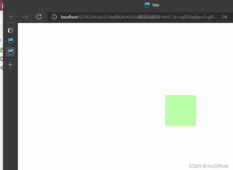
Js- get the mouse coordinates and follow them

Ubuntu 20.04 installing mysql8.0 and modifying the MySQL password

Sequential programming 1

System Verilog - thread
【Try to Hack】vulnhub DC1
随机推荐
SPARQL learning notes of query, an rrdf query language
Is it safe to open a stock account online?
Yolov4 coco pre train Darknet weight file
Ubuntu 20.04 installing mysql8.0 and modifying the MySQL password
The robot is playing an old DOS based game
C language LNK2019 unresolved external symbols_ Main error
What moment makes you think there is a bug in the world?
Brain tree (I)
Study notes of cmake
How to crop GIF dynamic graph? Take this picture online clipping tool
Installing QT plug-in in Visual Studio
Flexible layout (display:flex;) Attribute details
Some usage records about using pyqt5
One question per day,
Is it normal to dig for money? Is it safe to open a stock account?
One code per day - day one
Disable scrolling in the iPhone web app- Disable scrolling in an iPhone web application?
搭建极简GB28181 网守和网关服务器,建立AI推理和3d服务场景,然后开源代码(一)
Daily question, magic square simulation
basic_ String mind map