当前位置:网站首页>Common formulas of probability theory
Common formulas of probability theory
2022-07-03 09:20:00 【fishfuck】
Chapter one
The addition formula
P ( A ∪ B ) = P ( A ) + P ( B ) − P ( A B ) P(A \cup B)=P(A) + P(B)-P(AB) P(A∪B)=P(A)+P(B)−P(AB)
And so on ( Classical pattern )
P ( A ) = k n = A in package contain Of things Pieces of Count S in The base Ben things Pieces of Of total Count P(A)=\frac kn=\frac{A Number of events contained in }{S The total number of basic events in } P(A)=nk=S in The base Ben things Pieces of Of total Count A in package contain Of things Pieces of Count
Hypergeometric distribution
P = C D k C N D n − k C N n P = \frac{C_D^kC_{N_D}^{n-k}}{C_N^n} P=CNnCDkCNDn−k
event A The occurrence of a conditional event B Probability of occurrence
P ( B ∣ A ) = P ( A B ) P ( A ) P(B|A)=\frac {P(AB)}{P(A)} P(B∣A)=P(A)P(AB)
set up B 1 , B 2 … B_1,B_2\dots B1,B2… Not compatible with each other , Yes
P ( ⋃ i = 1 ∞ B i ∣ A ) = ∑ i = 1 ∞ P ( B i ∣ A ) P(\bigcup\limits_{i = 1}^\infty { {B_i}|A} ) = \sum\limits_{i = 1}^\infty {P({B_i}|A)} P(i=1⋃∞Bi∣A)=i=1∑∞P(Bi∣A)
Such as
P ( B 1 ∪ B 2 ∣ A ) = P ( B 1 ∣ A ) P ( A ) + P ( B 2 ∣ A ) P ( A ) − P ( B 1 B 2 ) ∣ P ( A ) P(B_1\cup B_2|A)=P(B_1|A)P(A)+P(B_2|A)P(A)-P(B_1B_2)|P(A) P(B1∪B2∣A)=P(B1∣A)P(A)+P(B2∣A)P(A)−P(B1B2)∣P(A)
Multiplication principle
P ( A B ) = P ( B ∣ A ) P ( A ) P(AB)=P(B|A)P(A) P(AB)=P(B∣A)P(A)
set up B 1 , B 2 , ⋯ , B n B_1,B_2,\cdots,B_n B1,B2,⋯,Bn Is the sample space S S S A division of , Then there are
All probability formula
P ( A ) = P ( A ∣ B 1 ) P ( B 1 ) + P ( A ∣ B 2 ) P ( B 2 ) + ⋯ + P ( A ∣ B n ) P ( B n ) P(A)=P(A|B_1)P(B_1)+P(A|B_2)P(B_2)+\cdots +P(A|B_n)P(B_n) P(A)=P(A∣B1)P(B1)+P(A∣B2)P(B2)+⋯+P(A∣Bn)P(Bn)
Bayes' formula
P ( B i ∣ A ) = P ( A ∣ B i ) P ( B i ) ∑ j = 1 n P ( A ∣ B j ) P ( B j ) P({B_i}|A) = \frac{ {P(A|{B_i})P({B_i})}}{ {\sum\limits_{j = 1}^n {P(A|{B_j})P({B_j})} }} P(Bi∣A)=j=1∑nP(A∣Bj)P(Bj)P(A∣Bi)P(Bi)
Special , When n = 2 n=2 n=2 when ,
P ( A ) = P ( A ∣ B ) P ( B ) + P ( A ∣ B ‾ ) P ( B ‾ ) P(A)=P(A|B)P(B)+P(A|\overline B)P(\overline B) P(A)=P(A∣B)P(B)+P(A∣B)P(B)
P ( B ∣ A ) = P ( A B ) P ( A ) = P ( A ∣ B ) P ( B ) P ( A ∣ B ) P ( B ) + P ( A ∣ B ‾ ) P ( B ‾ ) P({B}|A) =\frac {P(AB)}{P(A)}= \frac{ {P(A|{B})P({B})}}{P(A|B)P(B)+P(A|\overline B)P(\overline B)} P(B∣A)=P(A)P(AB)=P(A∣B)P(B)+P(A∣B)P(B)P(A∣B)P(B)
A 、 B A、B A、B When they are independent of each other , Yes
P ( A B ) = P ( B ∣ A ) P ( A ) = P ( A ) P ( B ) P(AB)=P(B|A)P(A)=P(A)P(B) P(AB)=P(B∣A)P(A)=P(A)P(B)
from n n n There is no put back extraction in different elements m m m Arrange the elements into An orderly column when , obtain
A n m = n ! ( n − m ) ! A_n^m=\frac {n!}{(n-m)!} Anm=(n−m)!n!
A different arrangement
from n n n There is no put back extraction in different elements m m m Elements Form a group regardless of order when , obtain
C n m = n ! m ! ( n − m ) ! C_n^m=\frac {n!}{m!(n-m)!} Cnm=m!(n−m)!n!
Two different combinations
if A ⊂ B A\subset B A⊂B( Notice the big decrease ), be
P ( B − A ) = P ( B ) − P ( A ) P(B-A)=P(B)-P(A) P(B−A)=P(B)−P(A)
Independent and Compatible with It could happen at the same time
13/11/2021 09:56
Chapter two
Discrete random variables : All possible values are finite or infinite
The binomial distribution (n Heavy Bernoulli experiment ): X ∼ b ( n , p ) X\sim b(n, p) X∼b(n,p)
P { X = k } = C n k p k q n − k , k = 0 , 1 , 2 , ⋯ , n P\{X=k\}=C^k_np^kq^{n-k},k=0, 1,2,\cdots,n P{ X=k}=Cnkpkqn−k,k=0,1,2,⋯,n
among q = 1 − p q=1-p q=1−p
When n = 2 n=2 n=2 when , The binomial distribution becomes 0-1 Distribution :
P { X = k } = p k ( 1 − p ) 1 − k , k = 0 , 1 P\{X=k\}=p^k(1-p)^{1-k},k=0, 1 P{ X=k}=pk(1−p)1−k,k=0,1
Poisson distribution : X ∼ π ( λ ) X\sim \pi(\lambda) X∼π(λ)
P { X = k } = λ k e − λ k ! P\{ X = k\} = \frac{ { {\lambda ^k}{e^{ - \lambda }}}}{ {k!}} P{ X=k}=k!λke−λ
When n Big enough ,p Enough hours , The binomial distribution can be estimated by Poisson distribution , There is a
C n k p k ( 1 − p ) n − k ≈ λ k e − λ k ! C_n^k{p^k}{(1 - p)^{n - k}} \approx \frac{ { {\lambda ^k}{e^{ - \lambda }}}}{ {k!}} Cnkpk(1−p)n−k≈k!λke−λ
among λ = n p \lambda =np λ=np
Distribution function
F ( x ) = P { X ≤ x } , − ∞ < x < + ∞ F(x)=P\{X\leq x\},-\infty <x<+\infty F(x)=P{ X≤x},−∞<x<+∞
For any real number x 1 < x 2 x_1<x_2 x1<x2, Yes
P { x 1 < X ≤ x 2 } = P { X ≤ x 2 } − P { X ≤ x 1 } = F ( x 2 ) − F ( x 1 ) P\{x_1<X\leq x_2\}=P\{X\leq x_2\}-P\{X\leq x_1\}=F(x_2)-F(x_1) P{ x1<X≤x2}=P{ X≤x2}−P{ X≤x1}=F(x2)−F(x1)
This property can be used to prove that the distribution function is an undiminished function
Continuous random variable : Distribution function F ( x ) F(x) F(x) Satisfy
F ( x ) = ∫ − ∞ x f ( t ) d t F(x) = \int_{ - \infty }^x {f(t)dt} F(x)=∫−∞xf(t)dt
call f ( x ) f(x) f(x) by X X X The probability density function of , abbreviation Probability density
Yes :
P { x 1 < X ≤ x 2 } = F ( x 2 ) − F ( x 1 ) = ∫ x 1 x 2 f ( x ) d x P\{x_1<X\leq x_2\}=F(x_2)-F(x_1)=\int _{x_1}^{x_2}f(x)dx P{ x1<X≤x2}=F(x2)−F(x1)=∫x1x2f(x)dx
F ′ ( x ) = f ( x ) F'(x)=f(x) F′(x)=f(x)
For continuous random variables , The probability of a single point is 0, That is to say
P { X = a } = 0 P\{X=a\}=0 P{ X=a}=0
Uniform distribution X ∼ U ( a , b ) X\sim U(a, b) X∼U(a,b):
f ( x ) = { 1 b − a , a < x < b 0 , Its He f(x)=\left\{ \begin{array}{lr} \frac 1{b-a}, & a<x<b \\ 0, & other \\ \end{array} \right. f(x)={ b−a1,0,a<x<b Its He
F ( x ) = { 0 , x < a x − a b − a , a ≤ x < b 1 , x ≥ b F(x)=\left\{ \begin{array}{lr} 0,&x<a\\ \frac {x-a}{b-a}, & a\leq x<b \\ 1, & x\geq b\\ \end{array} \right. F(x)=⎩⎨⎧0,b−ax−a,1,x<aa≤x<bx≥b
An index distribution :
f ( x ) = { 1 θ e − x θ , x > 0 0 , Its He f(x)=\left\{ \begin{array}{lr} \frac 1\theta e^{-\frac x\theta}, & x>0 \\ 0, & other \\ \end{array} \right. f(x)={ θ1e−θx,0,x>0 Its He
F ( x ) = { 1 − e − x θ , x > 0 0 , Its He F(x)=\left\{ \begin{array}{lr} 1-e^{-\frac x\theta}, & x>0 \\ 0, & other \\ \end{array} \right. F(x)={ 1−e−θx,0,x>0 Its He
Exponential distribution has no memory , That is to say :
P { X > s + t ∣ X > s } = P { x > t } P\{X>s+t|X>s\}=P\{x>t\} P{ X>s+t∣X>s}=P{ x>t}
Normal distribution : X ∼ N ( μ , σ 2 ) X\sim N(\mu , \sigma^2) X∼N(μ,σ2)
f ( x ) = 1 2 π σ e − ( x − μ ) 2 2 σ 2 , − ∞ < x < + ∞ f(x) = \frac{1}{ {\sqrt {2\pi } \sigma }}{e^{ - \frac{ { { {(x - \mu )}^2}}}{ {2{\sigma ^2}}}}}, - \infty < x < + \infty f(x)=2πσ1e−2σ2(x−μ)2,−∞<x<+∞
F ( x ) = 1 2 π σ ∫ − ∞ x e − ( t − μ ) 2 2 σ 2 d t F(x) = \frac{1}{ {\sqrt {2\pi } \sigma }}\int_{ - \infty }^x { {e^{ - \frac{ { { {(t - \mu )}^2}}}{ {2{\sigma ^2}}}}}} dt F(x)=2πσ1∫−∞xe−2σ2(t−μ)2dt
Special , When μ = 0 , σ = 1 \mu =0,\sigma = 1 μ=0,σ=1 It is called random variable X X X obey Standard normal distribution , Its probability density and distribution function are respectively used φ ( x ) , Φ ( x ) \varphi(x),\varPhi(x) φ(x),Φ(x) Express , Yes
φ ( x ) = 1 2 π σ e − x 2 2 , − ∞ < x < + ∞ \varphi(x) = \frac{1}{ {\sqrt {2\pi } \sigma }}{e^{ - \frac{x^2}2}}, - \infty < x < + \infty φ(x)=2πσ1e−2x2,−∞<x<+∞
Φ ( x ) = 1 2 π σ ∫ − ∞ x e − t 2 2 d t \varPhi(x) = \frac{1}{ {\sqrt {2\pi } \sigma }}\int_{ - \infty }^x { {e^{ - \frac{t^2}2}}} dt Φ(x)=2πσ1∫−∞xe−2t2dt
obviously , Yes
Φ ( − x ) = 1 − Φ ( x ) \varPhi(-x)=1-\varPhi(x) Φ(−x)=1−Φ(x)
If there are random variables X ∼ N ( μ , σ 2 ) X\sim N(\mu , \sigma^2) X∼N(μ,σ2), Then there are random variables Z, bring
Z = X − μ σ ∼ N ( 0 , 1 ) Z=\frac {X-\mu}\sigma \sim N(0,1) Z=σX−μ∼N(0,1)
When solving the distribution of the function of random variables , A more general method is to first deform by inequality F X ( x ) F_X(x) FX(x) or f X ( x ) f_X(x) fX(x) solve F Y ( y ) F_Y(y) FY(y), Right again F Y ( y ) F_Y(y) FY(y) Take the derivative and get f Y ( y ) f_Y(y) fY(y)
if X X X With probability density f X ( x ) , − ∞ < x < + ∞ f_X(x),-\infty<x<+\infty fX(x),−∞<x<+∞, And set up X X X To Y Y Y Transformation of Y = g ( X ) Y=g(X) Y=g(X) You can lead everywhere , Monotonous everywhere , be Y Y Y Probability density of
f Y ( y ) = { f X [ h ( y ) ] ∣ h ′ ( y ) ∣ , α < y < β 0 , Its He f_Y(y)=\left\{ \begin{array}{lr} f_X[h(y)]|h'(y)|, & \alpha<y<\beta \\ 0, & other \\ \end{array} \right. fY(y)={ fX[h(y)]∣h′(y)∣,0,α<y<β Its He
among h ( y ) h(y) h(y) yes g ( x ) g(x) g(x) The inverse function of
If there are random variables X ∼ N ( μ , σ 2 ) X\sim N(\mu , \sigma^2) X∼N(μ,σ2), Then its linear function Y = a X + b Y=aX+b Y=aX+b It also follows a normal distribution
13/11/2021 16:14
The third chapter
( For the conclusion of symmetry , Just give one , Another similar conclusion can be drawn )
Joint distribution function : set up ( X , Y ) (X,Y) (X,Y) It's a two-dimensional random variable , For any real number x x x, y y y, Dual function
F ( x , y ) = P { ( X ≤ x ) ∩ ( Y ≤ y ) } = P { X ≤ x , Y ≤ y } F(x,y)=P\{(X\leq x)\cap(Y\leq y) \}=P\{X\leq x, Y\leq y\} F(x,y)=P{ (X≤x)∩(Y≤y)}=P{ X≤x,Y≤y}
by ( X , Y ) (X,Y) (X,Y) The joint distribution function of
Joint distribution can be understood as ( X , Y ) (X,Y) (X,Y) The probability surrounded by the point to the infinite distance at the bottom left .
Yes
0 ≤ F ( x , y ) ≤ 1 0\leq F(x, y)\leq1 0≤F(x,y)≤1
∀ solid set Of y , F ( − ∞ , y ) = 0 \forall fixed y,F(-\infty,y)=0 ∀ solid set Of y,F(−∞,y)=0
∀ solid set Of x , F ( x , − ∞ ) = 0 \forall fixed x,F(x,-\infty)=0 ∀ solid set Of x,F(x,−∞)=0
F ( − ∞ , − ∞ ) = 0 , F ( + ∞ , + ∞ ) = 1 F(-\infty,-\infty)=0,F(+\infty,+\infty)=1 F(−∞,−∞)=0,F(+∞,+∞)=1
about ∀ ( x 1 , y 1 ) , ( x 2 , y 2 ) , x 1 < x 2 , y 1 < y 2 \forall(x_1,y_1),(x_2,y_2),x_1<x_2,y_1<y_2 ∀(x1,y1),(x2,y2),x1<x2,y1<y2, Yes
F ( x 2 , y 2 ) − F ( x 2 , y 1 ) + F ( x 1 , y 1 ) − F ( x 1 , y 2 ) ≥ 0 F(x_2,y_2)-F(x_2,y_1)+F(x_1,y_1)-F(x_1,y_2)\geq0 F(x2,y2)−F(x2,y1)+F(x1,y1)−F(x1,y2)≥0
14/11/2021 16:02
Two dimensional discrete random variables : Two-dimensional random variable ( X , Y ) (X,Y) (X,Y) All possible values are finite pairs or countable infinite pairs
Joint distribution law of two-dimensional random variables : P { X = x i , Y = y i } = p i j , i , j = 1 , 2 , ⋯ P\{X=x_i,Y=y_i\}=p_{ij},i,j=1,2,\cdots P{ X=xi,Y=yi}=pij,i,j=1,2,⋯
Or use a table to show
[ Failed to transfer the external chain picture , The origin station may have anti-theft chain mechanism , It is suggested to save the pictures and upload them directly (img-nKddJcCx-1637058108176)(:/c4a60e283b3243a3a2f472358ccdfb14)]
Two dimensional continuous random variables : If there is a nonnegative integrable function , send
F ( x , y ) = ∫ − ∞ y ∫ − ∞ x f ( u , v ) d u d v F(x,y) = \int_{ - \infty }^y {\int_{ - \infty }^x {f(u,v)dudv} } F(x,y)=∫−∞y∫−∞xf(u,v)dudv
be ( X , Y ) (X,Y) (X,Y) It is a two-dimensional continuous random variable , f ( x , y ) f(x,y) f(x,y) Is the probability density
Yes :
∫ − ∞ + ∞ ∫ − ∞ + ∞ f ( x , y ) d x d y = F ( + ∞ , + ∞ ) = 1 \int_{ - \infty }^{ + \infty } {\int_{ - \infty }^{ + \infty } {f(x,y)dxdy = F( + \infty , + \infty ) = 1} } ∫−∞+∞∫−∞+∞f(x,y)dxdy=F(+∞,+∞)=1
∂ 2 F ( x , y ) ∂ x ∂ y = f ( x , y ) \frac{ { {\partial ^2}F(x,y)}}{ {\partial x\partial y}} = f(x,y) ∂x∂y∂2F(x,y)=f(x,y)
Yes x O y xOy xOy The area on the plane G G G, Yes
P { ( X , Y ) ∈ G } = ∬ G f ( x , y ) d x d y P\{ (X,Y) \in G\} = \iint\limits_G {f(x,y)dxdy} P{ (X,Y)∈G}=G∬f(x,y)dxdy
Edge distribution function : Make a variable tend to infinity in the distribution function
F X ( x ) = F ( x , ∞ ) F_X(x)=F(x, \infty) FX(x)=F(x,∞)
F Y ( y ) = F ( ∞ , y ) F_Y(y)=F(\infty, y) FY(y)=F(∞,y)
Marginal distribution law of discrete random variables :
p i ⋅ = ∑ j = 1 ∞ p i j = P { X = x i } {p_{i\cdot}} = \sum\limits_{j = 1}^\infty { {p_{ij}}} = P\{ X = {x_i}\} pi⋅=j=1∑∞pij=P{ X=xi}
Edge distribution function of continuous random variables :
F X ( x ) = F ( x , ∞ ) = ∫ − ∞ x [ ∫ − ∞ ∞ f ( x , y ) d y ] d x {F_X}(x) = F(x,\infty ) = \int_{ - \infty }^x {[\int_{ - \infty }^\infty {f(x,y)dy} ]} dx FX(x)=F(x,∞)=∫−∞x[∫−∞∞f(x,y)dy]dx
Marginal probability density of continuous random variables :
f X ( x ) = ∫ − ∞ ∞ f ( x , y ) d y {f_X}(x) = \int_{ - \infty }^\infty {f(x,y)dy} fX(x)=∫−∞∞f(x,y)dy
stay Y = y i Y=y_i Y=yi( fixed ) Random variables under conditions X X X Conditional distribution law of :
P { X = x i ∣ Y = y j } = P { X = x i , Y = y i } P { Y = y i } = p i j p ⋅ j P\{X=x_i|Y=y_j\}=\frac {P\{X=x_i,Y=y_i\}}{P\{Y=y_i\}}=\frac {p_{ij}}{p_{\cdot j}} P{ X=xi∣Y=yj}=P{ Y=yi}P{ X=xi,Y=yi}=p⋅jpij
Conditional probability density of continuous random variables :
f X ∣ Y ( x ∣ y ) = f ( x , y ) f Y ( y ) f_{X|Y}(x|y)=\frac {f(x, y)}{f_Y(y)} fX∣Y(x∣y)=fY(y)f(x,y)
Conditional distribution function of continuous random variables :
F X ∣ Y ( x ∣ y ) = P { X ⩽ x ∣ Y = y } = ∫ − ∞ x f ( x , y ) f Y ( y ) d y {F_{X|Y}}(x|y) = P\{ X \leqslant x|Y = y\} = \int_{ - \infty }^x {\frac{ {f(x,y)}}{ { {f_Y}(y)}}dy} FX∣Y(x∣y)=P{ X⩽x∣Y=y}=∫−∞xfY(y)f(x,y)dy
Uniform distribution of two-dimensional random variables :
f ( x , y ) = { 1 A , ( x , y ) ∈ G 0 , Its He f(x,y)=\left\{ \begin{array}{lr} \frac 1A, &( x,y)\in G \\ 0, & other \\ \end{array} \right. f(x,y)={ A1,0,(x,y)∈G Its He
among G G G Is a bounded region on a plane , Area is A A A
Independent random variables
F ( x , y ) = F X ( x ) F Y ( y ) F(x,y)=F_X(x)F_Y(y) F(x,y)=FX(x)FY(y)
For continuous random variables , also
f ( x , y ) = f X ( x ) f Y ( y ) f(x,y)=f_X(x)f_Y(y) f(x,y)=fX(x)fY(y)
For two random variables :
Z = X + Y Z=X+Y Z=X+Y when
f X + Y ( z ) = ∫ − ∞ ∞ f ( z − y , y ) d y f_{X+Y}(z)=\int_{-\infty}^\infty f(z-y,y)dy fX+Y(z)=∫−∞∞f(z−y,y)dy
if X X X, Y Y Y Are independent of each other
f X + Y ( z ) = ∫ − ∞ ∞ f X ( z − y ) f Y ( y ) d y f_{X+Y}(z)=\int_{-\infty}^\infty f_X(z-y)f_Y(y)dy fX+Y(z)=∫−∞∞fX(z−y)fY(y)dy
Z = Y X Z=\frac YX Z=XY or Z = X Y Z=XY Z=XY when
f Y X ( z ) = ∫ − ∞ ∞ ∣ x ∣ f ( x , x z ) d x f_{\frac YX}(z)=\int_{-\infty}^\infty|x|f(x,xz)dx fXY(z)=∫−∞∞∣x∣f(x,xz)dx
f X Y ( z ) = ∫ − ∞ ∞ 1 ∣ x ∣ f ( x , z x ) d x f_{XY}(z)=\int_{-\infty}^{\infty}\frac 1{|x|}f(x,\frac zx)dx fXY(z)=∫−∞∞∣x∣1f(x,xz)dx
When they are independent of each other
f Y X ( z ) = ∫ − ∞ ∞ ∣ x ∣ f X ( x ) f Y ( x z ) d x f_{\frac YX}(z)=\int_{-\infty}^\infty|x|f_X(x)f_Y(xz)dx fXY(z)=∫−∞∞∣x∣fX(x)fY(xz)dx
f X Y ( z ) = ∫ − ∞ ∞ 1 ∣ x ∣ f X ( x ) f Y ( z x ) d x f_{XY}(z)=\int_{-\infty}^{\infty}\frac 1{|x|}f_X(x)f_Y(\frac zx)dx fXY(z)=∫−∞∞∣x∣1fX(x)fY(xz)dx
M = m a x { X , Y } M=max\{X,Y\} M=max{ X,Y} and N = m i n { X , Y } N=min\{X,Y\} N=min{ X,Y}( important )
( When they are independent of each other )
F m a x ( z ) = F X ( z ) F Y ( z ) F_{max}(z)=F_{X}(z)F_Y(z) Fmax(z)=FX(z)FY(z)
F m i n ( z ) = 1 − [ 1 − F X ( z ) ] [ 1 − F Y ( z ) ] F_{min}(z)=1-[1-F_X(z)][1-F_Y(z)] Fmin(z)=1−[1−FX(z)][1−FY(z)]
Extension
Yes M = m a x { X 1 , X 2 , ⋯ , X n } M=max\{X_1,X_2,\cdots,X_n\} M=max{ X1,X2,⋯,Xn} and N = m i n { X 1 , X 2 , ⋯ , X n } N=min\{X_1, X_2, \cdots,X_n\} N=min{ X1,X2,⋯,Xn}
F m a x ( z ) = F X 1 ( z ) F X 2 ( z ) ⋯ F X n ( z ) F_{max}(z)=F_{X_1}(z)F_{X_2}(z)\cdots F_{X_n}(z) Fmax(z)=FX1(z)FX2(z)⋯FXn(z)
F m i n ( z ) = 1 − [ 1 − F X 1 ( z ) ] [ 1 − F X 2 ( z ) ] ⋯ [ 1 − F X n ( z ) ] F_{min}(z)=1-[1-F_{X_1}(z)][1-F_{X_2}(z)]\cdots [1-F_{X_n}(z)] Fmin(z)=1−[1−FX1(z)][1−FX2(z)]⋯[1−FXn(z)]
Homodistribution
F m a x ( z ) = [ F ( z ) ] n F_{max}(z)=[F(z)]^n Fmax(z)=[F(z)]n
F m i n ( z ) = 1 − [ 1 − F ( z ) ] n F_{min}(z)=1-[1-F(z)]^n Fmin(z)=1−[1−F(z)]n
15/11/2021 21:47
Chapter four
Mathematical expectation : The average value of the characterization variable
( discrete )
E ( X ) = ∑ k = 1 ∞ x k p k E(X)=\sum\limits_{k=1}^\infty x_kp_k E(X)=k=1∑∞xkpk
When the series of the distribution law ∑ k = 1 ∞ x k p k \sum\limits_{k=1}^\infty x_kp_k k=1∑∞xkpk It is true when it is absolutely convergent
( Continuous type )
E ( X ) = ∫ − ∞ ∞ x f ( x ) d x E(X)=\int^\infty_{-\infty}xf(x)dx E(X)=∫−∞∞xf(x)dx
When the probability density is integral ∫ − ∞ ∞ x f ( x ) d x \int^\infty_{-\infty}xf(x)dx ∫−∞∞xf(x)dx It is true when it is absolutely convergent
set up Y = g ( X ) Y=g(X) Y=g(X), g g g It's a continuous function
( discrete )
E ( Y ) = E [ g ( X ) ] = ∑ k = 1 ∞ g ( x k ) p k E(Y)=E[g(X)]=\sum\limits^\infty_{k=1}g(x_k)p_k E(Y)=E[g(X)]=k=1∑∞g(xk)pk
( Continuous type )
E ( Y ) = E [ g ( X ) ] = ∫ − ∞ ∞ g ( x ) f ( x ) d x E(Y)=E[g(X)]=\int_{-\infty}^\infty g(x)f(x)dx E(Y)=E[g(X)]=∫−∞∞g(x)f(x)dx
For random variables Z = g ( X , Y ) Z=g(X,Y) Z=g(X,Y), Z Z Z It's one-dimensional , Then you can apply the above formula , set up ( X , Y ) (X,Y) (X,Y) The probability density of is f ( x , y ) f(x,y) f(x,y), Yes :
E ( Z ) = E [ g ( X , Y ) ] = ∫ − ∞ ∞ ∫ − ∞ ∞ g ( x , y ) f ( x , y ) d x d y E(Z)=E[g(X,Y)]=\int_{-\infty}^\infty\int_{-\infty}^\infty g(x,y)f(x,y)dxdy E(Z)=E[g(X,Y)]=∫−∞∞∫−∞∞g(x,y)f(x,y)dxdy
Then the expectation of a single two-dimensional random variable can be regarded as Z = X Z=X Z=X, Thus there are :
E ( X ) = ∫ − ∞ ∞ ∫ − ∞ ∞ x f ( x , y ) d x d y E(X)=\int_{-\infty}^\infty\int_{-\infty}^\infty xf(x,y)dxdy E(X)=∫−∞∞∫−∞∞xf(x,y)dxdy
For discrete random variables , There are similar conclusions :
E ( Z ) = E [ g ( X , Y ) ] = ∑ j = 1 ∞ ∑ i = 1 ∞ g ( x i , y i ) p i j E(Z)=E[g(X,Y)]=\sum\limits^\infty_{j=1}\sum\limits^\infty_{i=1}g(x_i,y_i)p_{ij} E(Z)=E[g(X,Y)]=j=1∑∞i=1∑∞g(xi,yi)pij
( Are independent of each other )
E ( X Y ) = E ( X ) E ( Y ) E(XY)=E(X)E(Y) E(XY)=E(X)E(Y)
variance : Represent the deviation degree of the variable from the mean , In essence, it is the average E ( X ) E(X) E(X) Function of
D ( X ) = V a r ( X ) = E { [ X − E ( X ) ] 2 } D(X)=Var(X)=E\{[X-E(X)]^2\} D(X)=Var(X)=E{ [X−E(X)]2}
( discrete )
D ( X ) = ∑ k = 1 ∞ [ x k − E ( X ) ] 2 p k D(X)=\sum\limits_{k=1}^\infty[x_k-E(X)]^2p_k D(X)=k=1∑∞[xk−E(X)]2pk
( Continuous type )
D ( X ) = ∫ − ∞ ∞ [ x − E ( X ) ] 2 f ( x ) d x D(X)=\int^\infty_{-\infty}[x-E(X)]^2f(x)dx D(X)=∫−∞∞[x−E(X)]2f(x)dx
Yes :
D ( X ) = E ( X 2 ) − [ E ( X ) ] 2 D(X)=E(X^2)-[E(X)]^2 D(X)=E(X2)−[E(X)]2
The nature of variance :
- D ( C ) = 0 D(C)=0 D(C)=0
- D ( C X ) = C 2 D ( X ) D(CX)=C^2D(X) D(CX)=C2D(X), D ( X + C ) = D ( X ) D(X+C)=D(X) D(X+C)=D(X)
- D ( X + Y ) = D ( X ) + D ( Y ) + 2 E { [ X − E ( X ) ] [ Y − E ( Y ) ] } D(X+Y)=D(X)+D(Y)+2E\{[X-E(X)][Y-E(Y)]\} D(X+Y)=D(X)+D(Y)+2E{ [X−E(X)][Y−E(Y)]}
, Special , When X X X, Y Y Y When they are independent of each other , D ( X + Y ) = D ( X ) + D ( Y ) D(X+Y)=D(X)+D(Y) D(X+Y)=D(X)+D(Y) - D ( X ) = 0 ⇔ P { X = E ( X ) } = 1 D(X)=0\Leftrightarrow P\{X=E(X)\}=1 D(X)=0⇔P{ X=E(X)}=1
Chebyshev inequality : Set the random variable X X X, E ( X ) = μ E(X)=\mu E(X)=μ, D ( X ) = σ 2 D(X)=\sigma^2 D(X)=σ2, On the other hand ∀ ε > 0 \forall\varepsilon>0 ∀ε>0
P { ∣ X − μ ∣ ≥ ε } ≤ σ 2 ε 2 P\{|X-\mu|\geq\varepsilon\}\leq\frac{\sigma^2}{\varepsilon^2} P{ ∣X−μ∣≥ε}≤ε2σ2
Focus on the six distributions ( Memorize )
| Distribution | Distribution law / Probability density | E ( X ) E(X) E(X) | D ( X ) D(X) D(X) |
|---|---|---|---|
| (0-1) Distribution | P { X = k } = p k ( 1 − p ) 1 − k P\{X=k\}=p^k(1-p)^{1-k} P{ X=k}=pk(1−p)1−k k = 0 , 1 k=0,1 k=0,1 | p p p | p ( 1 − p ) p(1-p) p(1−p) |
| The binomial distribution X ∼ b ( n , p ) X\sim b(n,p) X∼b(n,p) | P { X = k } = C n k p k q n − k P\{X=k\}=C^k_np^kq^{n-k} P{ X=k}=Cnkpkqn−k k = 0 , 1 , 2 , ⋯ , n k=0, 1,2,\cdots,n k=0,1,2,⋯,n | n p np np | n p ( 1 − p ) np(1-p) np(1−p) |
| Poisson distribution X ∼ π ( λ ) X\sim \pi(\lambda) X∼π(λ) | P { X = k } = λ k e − λ k ! P\{ X = k\} = \frac{ { {\lambda ^k}{e^{ - \lambda }}}}{ {k!}} P{ X=k}=k!λke−λ | λ \lambda λ | λ \lambda λ |
| Uniform distribution X ∼ U ( a , b ) X\sim U(a,b) X∼U(a,b) | f ( x ) = { 1 b − a , a < x < b 0 , Its He f(x)=\left\{\begin{array}{lr}\frac 1{b-a}, & a<x<b \\ 0, & other \\ \end{array}\right. f(x)={ b−a1,0,a<x<b Its He | a + b 2 \frac{a+b}2 2a+b | ( b − a ) 2 12 \frac{(b-a)^2}{12} 12(b−a)2 |
| An index distribution | f ( x ) = { 1 θ e − x θ , x > 0 0 , Its He f(x)=\left\{\begin{array}{lr} \frac 1\theta e^{-\frac x\theta}, & x>0 \\ 0, & other \\ \end{array}\right. f(x)={ θ1e−θx,0,x>0 Its He | θ \theta θ | θ 2 \theta^2 θ2 |
| Normal distribution X ∼ N ( μ , σ 2 ) X\sim N(\mu,\sigma^2) X∼N(μ,σ2) | f ( x ) = 1 2 π σ e − ( x − μ ) 2 2 σ 2 f(x) = \frac{1}{ {\sqrt {2\pi } \sigma }}{e^{ - \frac{ { { {(x - \mu )}^2}}}{ {2{\sigma ^2}}}}} f(x)=2πσ1e−2σ2(x−μ)2 − ∞ < x < + ∞ - \infty < x < + \infty −∞<x<+∞ | μ \mu μ | σ 2 \sigma^2 σ2 |
covariance :
C o v ( X , Y ) = E { [ X − E ( X ) ] [ Y − E ( Y ) ] } Cov(X,Y)=E\{[X-E(X)][Y-E(Y)]\} Cov(X,Y)=E{ [X−E(X)][Y−E(Y)]}
The correlation coefficient :
ρ X Y = C o v ( X , Y ) D ( X ) D ( Y ) \rho_{XY}=\frac {Cov(X,Y)}{\sqrt {D(X)}\sqrt {D(Y)}} ρXY=D(X)D(Y)Cov(X,Y)
Yes :
C o v ( X , X ) = D ( X ) Cov(X,X)=D(X) Cov(X,X)=D(X)
C o v ( X , Y ) = E ( X Y ) − E ( X ) E ( Y ) Cov(X,Y)=E(XY)-E(X)E(Y) Cov(X,Y)=E(XY)−E(X)E(Y)
C o v ( a X , b Y ) = a b C o v ( X , Y ) Cov(aX,bY)=abCov(X,Y) Cov(aX,bY)=abCov(X,Y)
C o v ( X 1 + X 2 , Y ) = C o v ( X 1 , Y ) + C o v ( X 2 , Y ) Cov(X_1+X_2,Y)=Cov(X_1,Y)+Cov(X_2,Y) Cov(X1+X2,Y)=Cov(X1,Y)+Cov(X2,Y)
∣ ρ X Y ∣ ≤ 1 |\rho_{XY}|\leq1 ∣ρXY∣≤1
∣ ρ X Y ∣ = 1 ⇔ ∃ a , b ∈ R , P { Y = a + b X } = 1 |\rho_{XY}|=1\Leftrightarrow\exist a,b\in\mathbb{R},P\{Y=a+bX\}=1 ∣ρXY∣=1⇔∃a,b∈R,P{ Y=a+bX}=1
When ρ X Y = 0 \rho_{XY}=0 ρXY=0 when , call X X X and Y Y Y No ( linear ) relevant
Irrelevant and independent are different , Are independent of each other ⇒ \Rightarrow ⇒ Unrelated , Unrelated ⇏ \nRightarrow ⇏ Are independent of each other
But for two-dimensional normal distribution , Are independent of each other ⇔ \Leftrightarrow ⇔ Unrelated
边栏推荐
- LeetCode 1089. Duplicate zero
- LeetCode 532. K-diff number pairs in array
- 【点云处理之论文狂读经典版12】—— FoldingNet: Point Cloud Auto-encoder via Deep Grid Deformation
- Basic knowledge of network security
- Common penetration test range
- 我們有個共同的名字,XX工
- With low code prospect, jnpf is flexible and easy to use, and uses intelligence to define a new office mode
- [untitled] use of cmake
- PIC16F648A-E/SS PIC16 8位 微控制器,7KB(4Kx14)
- [graduation season | advanced technology Er] another graduation season, I change my career as soon as I graduate, from animal science to programmer. Programmers have something to say in 10 years
猜你喜欢
![[point cloud processing paper crazy reading classic version 12] - foldingnet: point cloud auto encoder via deep grid deformation](/img/62/edb888200e3743b03e5b39d94758f8.png)
[point cloud processing paper crazy reading classic version 12] - foldingnet: point cloud auto encoder via deep grid deformation

Go language - Reflection
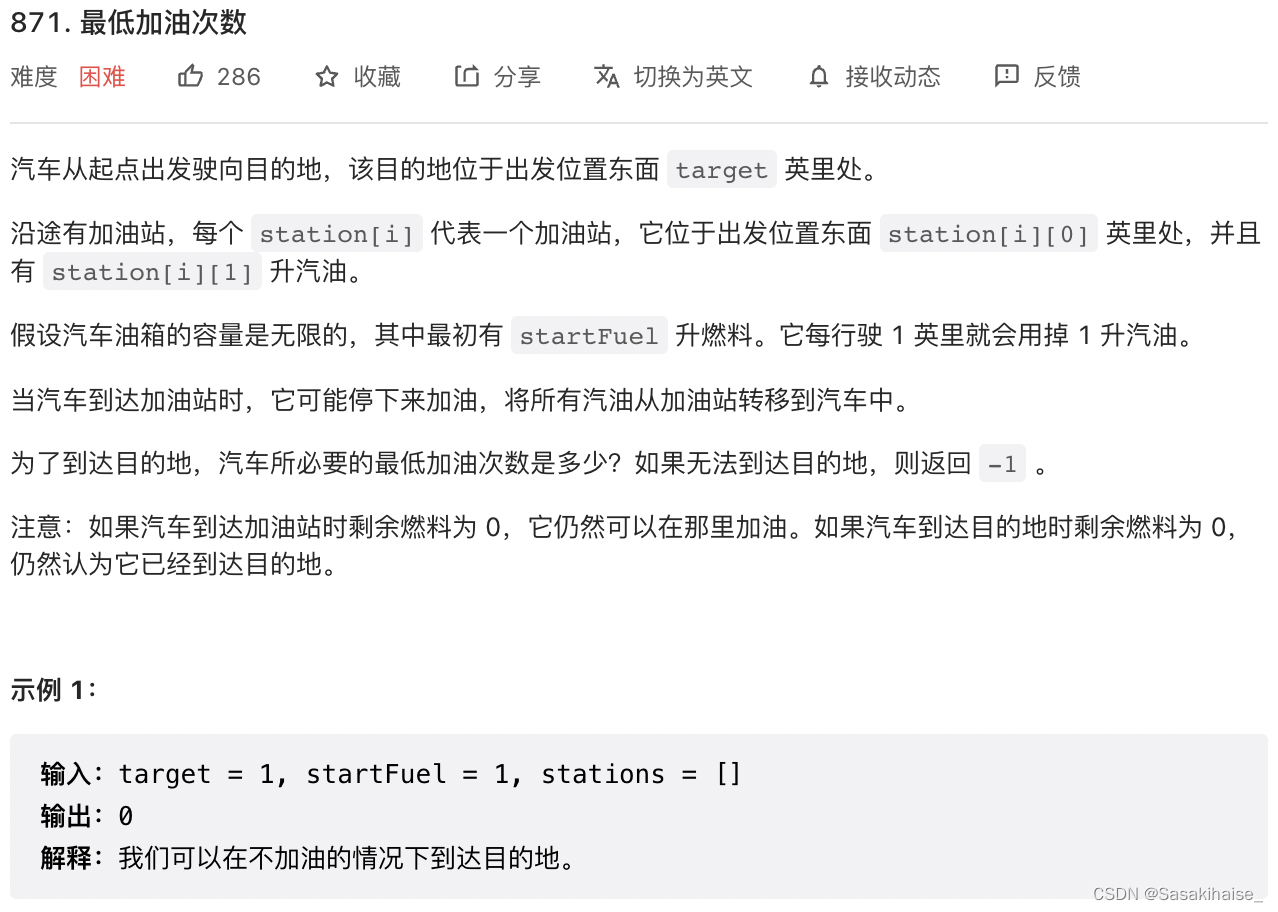
LeetCode 871. 最低加油次数

Common penetration test range

What is an excellent fast development framework like?

Sword finger offer II 029 Sorted circular linked list
![[point cloud processing paper crazy reading frontier edition 13] - gapnet: graph attention based point neural network for exploring local feature](/img/66/2e7668cfed1ef4ddad26deed44a33a.png)
[point cloud processing paper crazy reading frontier edition 13] - gapnet: graph attention based point neural network for exploring local feature

数字化转型中,企业设备管理会出现什么问题?JNPF或将是“最优解”
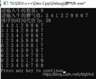
Temper cattle ranking problem

我们有个共同的名字,XX工
随机推荐
With low code prospect, jnpf is flexible and easy to use, and uses intelligence to define a new office mode
AcWing 788. Number of pairs in reverse order
The difference between if -n and -z in shell
Jenkins learning (II) -- setting up Chinese
Beego learning - Tencent cloud upload pictures
我們有個共同的名字,XX工
Methods of using arrays as function parameters in shell
[point cloud processing paper crazy reading classic version 8] - o-cnn: octree based revolutionary neural networks for 3D shape analysis
Jenkins learning (I) -- Jenkins installation
Noip 2002 popularity group selection number
Simple use of MATLAB
[point cloud processing paper crazy reading cutting-edge version 12] - adaptive graph revolution for point cloud analysis
【点云处理之论文狂读前沿版9】—Advanced Feature Learning on Point Clouds using Multi-resolution Features and Learni
LeetCode 532. 数组中的 k-diff 数对
【点云处理之论文狂读前沿版12】—— Adaptive Graph Convolution for Point Cloud Analysis
[point cloud processing paper crazy reading frontier version 10] - mvtn: multi view transformation network for 3D shape recognition
LeetCode 715. Range module
2022-1-6 Niuke net brush sword finger offer
[point cloud processing paper crazy reading classic version 11] - mining point cloud local structures by kernel correlation and graph pooling
常见渗透测试靶场