What can the graph of training and verification indicators tell us in machine learning?

When we train and verify the model, we will save the training indicators and make them into charts , In this way, you can view and analyze after you finish , But do you really understand the meaning of these indicators ？

In this article, we will summarize the possible situations of training and verification and introduce what kind of information these charts can provide us .

Let's start with some simple code , The following code establishes a basic training process framework .

from sklearn.model_selection import train_test_split
from sklearn.datasets import  make_classification
import torch
from torch.utils.data import Dataset, DataLoader
import torch.optim as torch_optim
import torch.nn as nn
import torch.nn.functional as F
import numpy as np
import matplotlib.pyplot as pltclass MyCustomDataset(Dataset):
    def __init__(self, X, Y, scale=False):
        self.X = torch.from_numpy(X.astype(np.float32))
        self.y = torch.from_numpy(Y.astype(np.int64))
    
    def __len__(self):
        return len(self.y)
    
    def __getitem__(self, idx):
        return self.X[idx], self.y[idx]def get_optimizer(model, lr=0.001, wd=0.0):
    parameters = filter(lambda p: p.requires_grad, model.parameters())
    optim = torch_optim.Adam(parameters, lr=lr, weight_decay=wd)
    return optimdef train_model(model, optim, train_dl, loss_func):
    # Ensure the model is in Training mode
    model.train()
    total = 0
    sum_loss = 0
    for x, y in train_dl:
        batch = y.shape[0]
        # Train the model for this batch worth of data
        logits = model(x)
        # Run the loss function. We will decide what this will be when we call our Training Loop
        loss = loss_func(logits, y)
        # The next 3 lines do all the PyTorch back propagation goodness
        optim.zero_grad()
        loss.backward()
        optim.step()
        # Keep a running check of our total number of samples in this epoch
        total += batch
        # And keep a running total of our loss
        sum_loss += batch*(loss.item())
    return sum_loss/total
def train_loop(model, train_dl, valid_dl, epochs, loss_func, lr=0.1, wd=0):
    optim = get_optimizer(model, lr=lr, wd=wd)
    train_loss_list = []
    val_loss_list = []
    acc_list = []
    for i in range(epochs): 
        loss = train_model(model, optim, train_dl, loss_func)
        # After training this epoch, keep a list of progress of 
        # the loss of each epoch 
        train_loss_list.append(loss)
        val, acc = val_loss(model, valid_dl, loss_func)
        # Likewise for the validation loss and accuracy
        val_loss_list.append(val)
        acc_list.append(acc)
        print("training loss: %.5f     valid loss: %.5f     accuracy: %.5f" % (loss, val, acc))
    
    return train_loss_list, val_loss_list, acc_list
def val_loss(model, valid_dl, loss_func):
    # Put the model into evaluation mode, not training mode
    model.eval()
    total = 0
    sum_loss = 0
    correct = 0
    batch_count = 0
    for x, y in valid_dl:
        batch_count += 1
        current_batch_size = y.shape[0]
        logits = model(x)
        loss = loss_func(logits, y)
        sum_loss += current_batch_size*(loss.item())
        total += current_batch_size
        # All of the code above is the same, in essence, to
        # Training, so see the comments there
        # Find out which of the returned predictions is the loudest
        # of them all, and that's our prediction(s)
        preds = logits.sigmoid().argmax(1)
        # See if our predictions are right
        correct += (preds == y).float().mean().item()
    return sum_loss/total, correct/batch_count
def view_results(train_loss_list, val_loss_list, acc_list):
    plt.rcParams["figure.figsize"] = (15, 5)
    plt.figure()
    epochs = np.arange(0, len(train_loss_list))    plt.subplot(1, 2, 1)
    plt.plot(epochs-0.5, train_loss_list)
    plt.plot(epochs, val_loss_list)
    plt.title('model loss')
    plt.ylabel('loss')
    plt.xlabel('epoch')
    plt.legend(['train', 'val', 'acc'], loc = 'upper left')
    
    plt.subplot(1, 2, 2)
    plt.plot(acc_list)
    plt.title('accuracy')
    plt.ylabel('accuracy')
    plt.xlabel('epoch')
    plt.legend(['train', 'val', 'acc'], loc = 'upper left')
    plt.show()
    
def get_data_train_and_show(model, batch_size=128, n_samples=10000, n_classes=2, n_features=30, val_size=0.2, epochs=20, lr=0.1, wd=0, break_it=False):
    # We'll make a fictitious dataset, assuming all relevant
    # EDA / Feature Engineering has been done and this is our 
    # resultant data
    X, y = make_classification(n_samples=n_samples, n_classes=n_classes, n_features=n_features, n_informative=n_features, n_redundant=0, random_state=1972)
    
    if break_it: # Specifically mess up the data
        X = np.random.rand(n_samples,n_features)
    X_train, X_val, y_train, y_val = train_test_split(X, y, test_size=val_size, random_state=1972)    train_ds = MyCustomDataset(X_train, y_train)
    valid_ds = MyCustomDataset(X_val, y_val)
    train_dl = DataLoader(train_ds, batch_size=batch_size, shuffle=True)
    valid_dl = DataLoader(valid_ds, batch_size=batch_size, shuffle=True)    train_loss_list, val_loss_list, acc_list = train_loop(model, train_dl, valid_dl, epochs=epochs, loss_func=F.cross_entropy, lr=lr, wd=wd)
    view_results(train_loss_list, val_loss_list, acc_list)

The above code is simple , It's about getting data , Training , Verify such a basic process , Now let's get to the point .

scene 1 - The model seems to be learnable , But poor performance in validation or accuracy

No matter what the super parameter is , Model Train loss Will slow down , but Val loss It won't fall , And its Accuracy It doesn't mean it's learning anything .

For example, in this case , The accuracy of binary classification hovers in 50% about .

class Scenario_1_Model_1(nn.Module):
    def __init__(self, in_features=30, out_features=2):
        super().__init__()
        self.lin1 = nn.Linear(in_features, out_features)
    def forward(self, x):
        x = self.lin1(x)
        return x

get_data_train_and_show(Scenario_1_Model_1(), lr=0.001, break_it=True)

There is not enough information in the data to allow ‘ Study ’, The training data may not contain enough information to make the model “ Study ”.

under these circumstances （ The training data in the code is random data ）, This means that it cannot learn any substance .

Data must have enough information to learn from .EDA And feature engineering is the key ！ What model learning can learn , Instead of making up something that doesn't exist .

scene 2 — Training 、 The validation and accuracy curves are very unstable

For example, the following code ：lr=0.1,bs=128

class Scenario_2_Model_1(nn.Module):
    def __init__(self, in_features=30, out_features=2):
        super().__init__()
        self.lin1 = nn.Linear(in_features, out_features)
    def forward(self, x):
        x = self.lin1(x)
        return x

get_data_train_and_show(Scenario_2_Model_1(), lr=0.1)

“ Learning rate is too high ” or “ The batch size is too small ” Try to reduce the learning rate from 0.1 Down to 0.001, That means it won't “ rebound ”, But it will decrease steadily .

get_data_train_and_show(Scenario_1_Model_1(), lr=0.001)

In addition to reducing the learning rate , Increasing the batch size will also make it smoother .

get_data_train_and_show(Scenario_1_Model_1(), lr=0.001, batch_size=256)

scene 3—— The training loss is close to zero , The accuracy looks good , But verification It didn't go down , And it went up

class Scenario_3_Model_1(nn.Module):
    def __init__(self, in_features=30, out_features=2):
        super().__init__()
        self.lin1 = nn.Linear(in_features, 50)
        self.lin2 = nn.Linear(50, 150)
        self.lin3 = nn.Linear(150, 50)
        self.lin4 = nn.Linear(50, out_features)
    def forward(self, x):
        x = F.relu(self.lin1(x))
        x = F.relu(self.lin2(x))
        x = F.relu(self.lin3(x))
        x = self.lin4(x)
        return x
get_data_train_and_show(Scenario_3_Model_1(), lr=0.001)

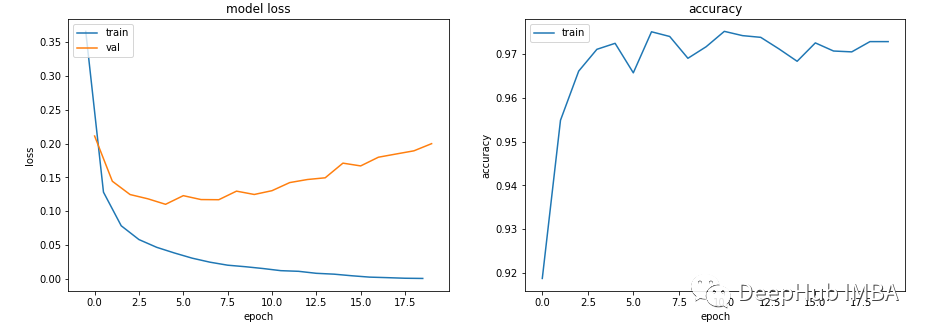
This must be a fitting ： Low training loss and high accuracy , And the loss of verification and training is getting larger and larger , Are classic over fitting indicators .

Basically , Your model learning ability is too strong . It has a good memory of training data , This means that it cannot be generalized to new data .

The first thing we can try is to reduce the complexity of the model .

class Scenario_3_Model_2(nn.Module):
    def __init__(self, in_features=30, out_features=2):
        super().__init__()
        self.lin1 = nn.Linear(in_features, 50)
        self.lin2 = nn.Linear(50, out_features)
    def forward(self, x):
        x = F.relu(self.lin1(x))
        x = self.lin2(x)
        return x

get_data_train_and_show(Scenario_3_Model_2(), lr=0.001)

This makes it better , You can also introduce L2 Weight attenuation regularization , Make it better again （ Suitable for shallow models ）.

get_data_train_and_show(Scenario_3_Model_2(), lr=0.001, wd=0.02)

If we want to keep the depth and size of the model , You can try to use dropout（ For deeper models ）.

class Scenario_3_Model_3(nn.Module):
    def __init__(self, in_features=30, out_features=2):
        super().__init__()
        self.lin1 = nn.Linear(in_features, 50)
        self.lin2 = nn.Linear(50, 150)
        self.lin3 = nn.Linear(150, 50)
        self.lin4 = nn.Linear(50, out_features)
        self.drops = nn.Dropout(0.4)
    def forward(self, x):
        x = F.relu(self.lin1(x))
        x = self.drops(x)
        x = F.relu(self.lin2(x))
        x = self.drops(x)
        x = F.relu(self.lin3(x))
        x = self.drops(x)
        x = self.lin4(x)
        return x
get_data_train_and_show(Scenario_3_Model_3(), lr=0.001)

scene 4 - Good training and verification , But the accuracy is not improved

lr = 0.001,bs = 128（ Default , Classification categories = 5

class Scenario_4_Model_1(nn.Module):
    def __init__(self, in_features=30, out_features=2):
        super().__init__()
        self.lin1 = nn.Linear(in_features, 2)
        self.lin2 = nn.Linear(2, out_features)
    def forward(self, x):
        x = F.relu(self.lin1(x))
        x = self.lin2(x)
        return x

get_data_train_and_show(Scenario_4_Model_1(out_features=5), lr=0.001, n_classes=5)

Not enough learning ability ： The parameters of one layer in the model are less than the classes in the possible output of the model . under these circumstances , When there is 5 Possible output classes , The only intermediate parameters are 2 individual .

This means that the model loses information , Because it has to fill it with a smaller layer , So once the layer parameters are expanded again , It is difficult to recover this information .

Therefore, the parameters of the recording layer should never be smaller than the output size of the model .

class Scenario_4_Model_2(nn.Module):
    def __init__(self, in_features=30, out_features=2):
        super().__init__()
        self.lin1 = nn.Linear(in_features, 50)
        self.lin2 = nn.Linear(50, out_features)
    def forward(self, x):
        x = F.relu(self.lin1(x))
        x = self.lin2(x)
        return x
get_data_train_and_show(Scenario_4_Model_2(out_features=5), lr=0.001, n_classes=5)

summary

These are some common exercises 、 Examples of curves at the time of validation , I hope you can quickly locate and improve in the same situation .

https://avoid.overfit.cn/post/5f52eb0868ce41a3a847783d5e87a04f

author ：Martin Keywood