【点云处理之论文狂读经典版11】—— Mining Point Cloud Local Structures by Kernel Correlation and Graph Pooling

摘要

• 问题： 点云的无序性(unorder)对于语义学习而言还是很有挑战性的，在现有的方法中，PointNet通过直接在点集上进行学习获得了不错的结果，但是PointNet并没有充分利用点云的局部邻域信息，点云的局部邻域信息中包含着fine-grained结构信息，能够有助于更好的语义学习。
• 方法： 提出了两种新的操作，以提高PointNet发掘局部结构的效率。
• 技术细节：
  ①第一种操作注重局部3D几何 (geometric) 结构，将point-set kernel定义成一组可学习的3D points，这些points对一组相邻点做出响应，通过 kernel correlation 测量这些相邻点间的几何关系
  ②第二种操作利用局部高维特征 (feature) 结构，通过点云的3D位置计算得到nearest-neighbor-graph，然后在nearest-neighbor-graph上递归地进行特征聚合 (feature aggregation) 实现该操作。
• 代码：
  ① http://www.merl.com/research/license#KCNet
  ② https://github.com/ftdlyc/KCNet_Pytorch PyTorch版本 可能运行不起来，是部分代码

引言

• PointNet直接将全部点的特征聚合为全局特征，表明PointNet并没有充分利用点的局部结构挖掘fine-grained patterns：每个点的MLP输出仅对3D空间的特定非线性分区中存在的3D点进行粗略编码。
• 如果MLP不仅可以对“wether”存在点进行编码，还可以对非线性3D空间分区中存在的点确定“what type of”（例如，角点与平面、凸点与凹点等）进行编码，则就是我们期望得到的更具区别性的表示。
• 这种“type”信息必须要从3D目标表面上点的局部领域中学习。
• 主要贡献：
  1. kernel correlation layer ——> 挖掘局部几何结构
  2. graph-based pooling layer ——>挖掘局部特征结构

方法

Learning on Local Geometric Structure

本文中，以点云的local neighborhood作为source，以可学习的kernel(一组点)作为reference，从而表示局部结构/形状的type。在点云配准任务中，source和reference中的点都是固定不动的，但是本文允许reference中的点发生变化，通过学习(反向传播)的方式去更加“贴合”形状。与点云配准不同的是，我们想要通过一种非变换的方式学习reference，而不是通过最优变换的方式。通过这种方式可学习的kernel点与卷积kernel就相同了，都是在相邻区域内对每个点作出响应，并且在这个感知域内捕获局部几何结构，这个感知域是通过kernel函数和kernel wedth决定的。通过这种配置，学习的过程可以看作是找到一组能够对最高效和最有用的局部几何结构进行编码的reference点，并联合网络中的其他参数获得最好的学习性能。

具体而言，定义带有$M$个可学习点的point-set kernel $\mathbf{\kappa }$和带有$N$ 个点的点云中的当前anchor point ${\mathbf{x}}_i$ 之间的 kernel correlation (KC) 为：
$$\mathrm{K}\mathrm{C}\left(\mathbf{\kappa },{\mathbf{x}}_i\right)=\frac{1}{|\mathcal{N}(i)|}\sum _{m=1}^M\sum _{n\in \mathcal{N}(i)}{\mathrm{K}}_{\sigma }\left({\mathbf{\kappa }}_m,{\mathbf{x}}_n-{\mathbf{x}}_i\right)$$
其中${\mathbf{\kappa }}_m$是kernel中的第$m$个可学习点，$\mathcal{N}(i)$ 是anchor point ${\mathbf{x}}_i$的邻域索引，${\mathbf{x}}_n$是${\mathbf{x}}_i$的一个neighbor point。${\mathrm{K}}_{\sigma }(\cdot ,\cdot ):{\Re }^D\times {\Re }^D\to$$\Re$是任意的kernel函数。为了有效存储点的局部邻域，我们将每个点作为顶点，仅相邻的顶点才会用边连接，从而提前构造一个KNNG。

在不失一般性的情况下，本文选择Gaussian kernel：
$$K_{\sigma }(\mathbf{k},\mathbf{\delta })=\exp \left(-\frac{\Vert \mathbf{k}-\mathbf{\delta }{\Vert }^2}{2{\sigma }^2}\right)$$
其中$\Vert \cdot \Vert$表示两个点之间的欧式距离，$\sigma$是kernel宽度，控制着点与点之间距离的影响。Gaussian kernel的一个很好的性质就是两个点之间的距离呈指数函数的趋势，还提供一个从每个kernel点到anchor point的neighbor points之间的soft-assignment(可导)。KC对kernel points 和 neighboring points之间的距离进行编码，并且增加两组点云在形状上的相似性。值得注意的是这里的kernel width，太大或者太小都会导致不理想的结果，可以通过实验进行选择。

给定：

1. 网络损失函数$\mathcal{L}$
2. 损失函数相对于每个anchor point ${\mathbf{x}}_i$的$\mathrm{K}\mathrm{C}$自顶层反向传播的导数$d_i=\frac{\partial \mathcal{L}}{\partial \mathrm{K}\mathrm{C}\left(\mathbf{\kappa },{\mathbf{x}}_i\right)}$

本文提供了每个kernel point ${\kappa }_m$的反向传播公式：
$$\frac{\partial \mathcal{L}}{\partial {\mathbf{\kappa }}_m}=\sum _{i=1}^N{\alpha }_i{d}_i\left[\sum _{n\in \mathcal{N}(i)}{\mathbf{v}}_{m,i,n}\exp \left(-\frac{{\Vert {\mathbf{v}}_{m,i,n}\Vert }^2}{2{\sigma }^2}\right)\right]$$
其中点$x_i$的归一化常数为${\alpha }_i=\frac{-1}{|\mathcal{N}(i)|{\sigma }^2}$，局部偏差向量为${\mathbf{v}}_{m,i,n}={\mathbf{\kappa }}_m+{\mathbf{x}}_i-{\mathbf{x}}_n$。

Learning on Local Feature Structure

$\mathrm{K}\mathrm{C}$仅仅是作用在网络的前端用于提取局部几何结构。在之前我们也讲过，通过构造KNNG来获取相邻点信息，这个graph还可以被用于在更深层中挖掘局部特征结构。受到卷积网络能够局部聚合特征，并且通过多个pooling层逐步增加感受野的启发，我们沿着3D neighborhood graph的边递归地进行特征传播和特征聚合，以便于在上层中提取局部特征。

我们的一个关键思想就是neighbor points更趋向于有着相似的几何结构，因此通过neighborhood graph传播特征能够帮助学习更鲁棒的局部patterns。值得注意的是，我们特地在上面的这些层中避免改变neighborhood graph的结构。

令 $\mathbf{X}\in {\Re }^{N\times K}$ 表示graph pooling的输入，那么KNNG有着邻接矩阵$\mathbf{W}\in$${\Re }^{N\times N}$，其中如果顶点$i$和顶点$j$之间存在一条边，那么$\mathbf{W}(i,j)=1$，否则$\mathbf{W}(i,j)=0$。直觉上讲，形成局部表面的neighboring points通常共享相似地特征pattern。因此，通过graph pooling操作在每个点的邻域内聚合特征：
$$\mathbf{Y}=\mathbf{P}\mathbf{X}$$
pooling操作可以是average pooling，也可以是max pooling。

Graph average pooling就是通过使用$\mathbf{P}\in {\Re }^{N\times N}$作为一个归一化邻接矩阵对一个点邻域内的所有特征取平均值：
$$\mathbf{P}={\mathbf{D}}^{-1}\mathbf{W},$$
其中$\mathbf{D}\in {\Re }^{N\times N}$是度矩阵，第$(i,j)$个entry $d_{i,j}$定义为：

$$d_{i,j}=\{\begin{array}{ll}\mathrm{deg}(i),& \text{ if }i=j\\ 0,& \text{ otherwise }\end{array}$$
其中$\mathrm{deg}(i)$是顶点$i$的度，表示所有连接到顶点$i$的顶点数量。

Graph max pooling(GM)取每个顶点邻域内的最大特征，在$K$个维度上单独操作。因此输出$\mathbf{Y}$的第$(i,k)$个entry为：
$$\mathbf{Y}(i,k)=\underset{n\in \mathcal{N}(i)}{\max }\mathbf{X}(n,k)$$
其中$\mathcal{N}(i)$表示点集${\mathbf{X}}_i$的邻居索引，从$\mathbf{W}$中计算得到。

实验

Shape Classification

Network Configuration

如上图所示，KCNet共有9层。值得注意的是，KNN-Group不参与训练，甚至可以提前计算好，它的作用就是构造相邻点和特征聚合，起到一个结构性的作用。

1. 第一层，kernel correlation，以点坐标作为输入，输出的是局部结构特征，并且和点坐标再进行拼接。
2. 然后特征通过第一次的两个MLP进行逐点的特征学习。
3. 接着graph pooling layer将输出的逐点特征聚合为更鲁棒的局部结构特征，再与第二次的两个MLP输出进行拼接。

剩下的结构跟PointNet很相似，除了 1)不使用Batchnorm，ReLU用在每个全连接的后面；2)Dropout用于最后的全连接层，值设置为0.5；

在kernel computation 和 graph max pooling中使用16-NN graph，kernel的数量$L$为32，每个kernel都有16个点，初始值设置为$[-0.2,0.2]$，kernel width$\sigma =0.005$。

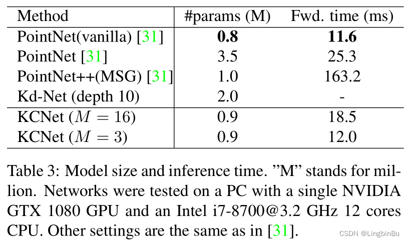
Results

Part Segmentation

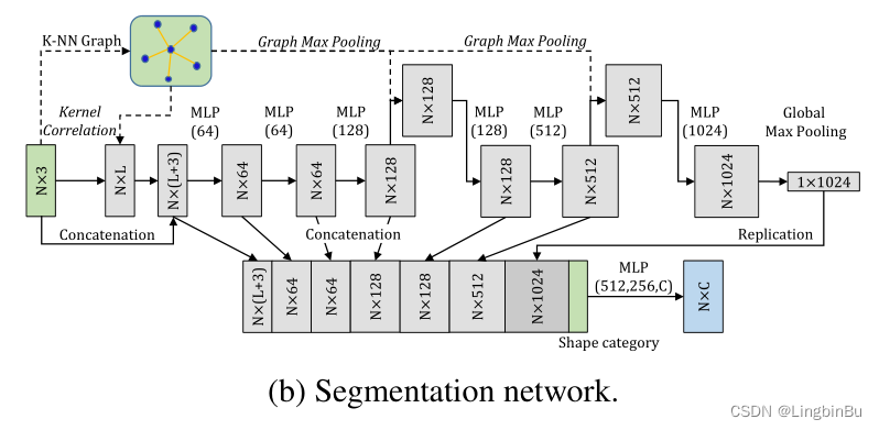
Network Configuration

语义网络有10层，不同层的特征捕获的局部特征会和全局特征与形状信息进行拼接。也没用到Batchnorm，Dropout层被用于全连接层，值为0.3。18-NN graph用于kernel computation 和 graph max pooling。kernel的数量为16，每个kernel中有18个点，初始值在$[-0.2,0.2]$之间，kernel width $\sigma =0.005$。

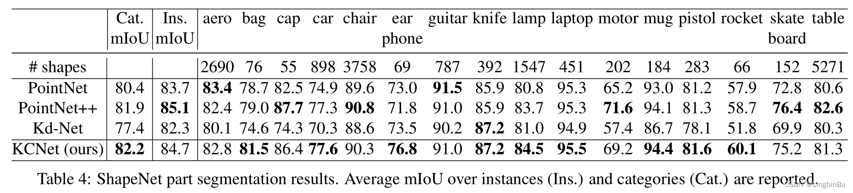
Results

Ablation Study

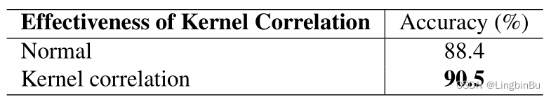
Effectiveness of Kernel Correlation

Symmetric Functions

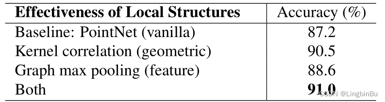
Effectiveness of Local Structures

Choosing Hyper-parameters

Robustness Test