Analysis of 43 cases of MATLAB neural network: Chapter 26 classification of LVQ Neural Network - breast tumor diagnosis

1. Preface

《MATLAB neural network 43 A case study 》 yes MATLAB Technology Forum （www.matlabsky.com） planning , Led by teacher wangxiaochuan ,2013 Beijing University of Aeronautics and Astronautics Press MATLAB A book for tools MATLAB Example teaching books , Is in 《MATLAB neural network 30 A case study 》 On the basis of modification 、 Complementary , Adhering to “ Theoretical explanation — case analysis — Application extension ” This feature , Help readers to be more intuitive 、 Learn neural networks vividly .

《MATLAB neural network 43 A case study 》 share 43 Chapter , The content covers common neural networks （BP、RBF、SOM、Hopfield、Elman、LVQ、Kohonen、GRNN、NARX etc. ） And related intelligent algorithms （SVM、 Decision tree 、 Random forests 、 Extreme learning machine, etc ）. meanwhile , Some chapters also cover common optimization algorithms （ Genetic algorithm (ga) 、 Ant colony algorithm, etc ） And neural network . Besides ,《MATLAB neural network 43 A case study 》 It also introduces MATLAB R2012b New functions and features of neural network toolbox in , Such as neural network parallel computing 、 Custom neural networks 、 Efficient programming of neural network, etc .

In recent years, with the rise of artificial intelligence research , The related direction of neural network has also ushered in another upsurge of research , Because of its outstanding performance in the field of signal processing , The neural network method is also being applied to various applications in the direction of speech and image , This paper combines the cases in the book , It is simulated and realized , It's a relearning , I hope I can review the old and know the new , Strengthen and improve my understanding and practice of the application of neural network in various fields . I just started this book on catching more fish , Let's start the simulation example , Mainly to introduce the source code application examples in each chapter , This paper is mainly based on MATLAB2015b(32 position ) Platform simulation implementation , This is Chapter 26 of the book LVQ Examples of neural network classification , Don't talk much , Start ！

2. MATLAB Simulation example

open MATLAB, Click on “ Home page ”, Click on “ open ”, Find the sample file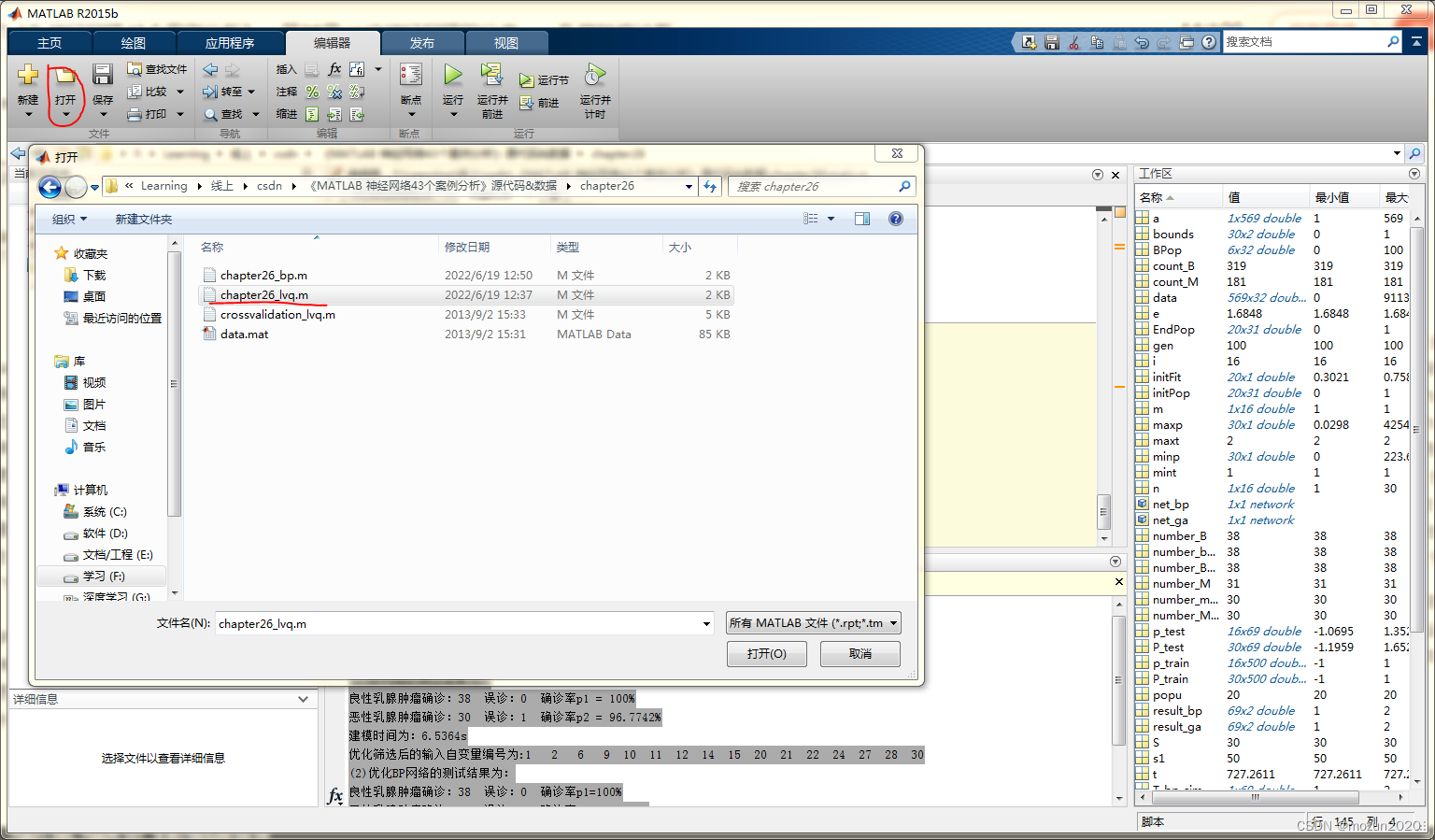

Choose chapter26_lvq.m, Click on “ open ”

chapter26_lvq.m Source code is as follows ：

%%%%%%%%%%%%%%%%%%%%%%%%%%%%%%%%%%%%%%%%%%%%%%%%%%%%
% function ： LVQ Classification of neural networks —— Breast tumor diagnosis 
% Environmental Science ：Win7,Matlab2015b
%Modi: C.S
% Time ：2022-06-18
%%%%%%%%%%%%%%%%%%%%%%%%%%%%%%%%%%%%%%%%%%%%%%%%%%%%


%% LVQ Classification of neural networks —— Breast tumor diagnosis 

%%  Clear environment variables 
clear all
clc
warning off
tic
%%  Import data 
load data.mat
a = randperm(569);
Train = data(a(1:500),:);
Test = data(a(501:end),:);
%  Training data 
P_train = Train(:,3:end)';
Tc_train = Train(:,2)';
T_train = ind2vec(Tc_train);
%  Test data 
P_test = Test(:,3:end)';
Tc_test = Test(:,2)';

%%  Creating networks 
count_B = length(find(Tc_train == 1));
count_M = length(find(Tc_train == 2));
rate_B = count_B/500;
rate_M = count_M/500;
net = newlvq(minmax(P_train),20,[rate_B rate_M],0.01,'learnlv1');
%  Set network parameters 
net.trainParam.epochs = 1000;
net.trainParam.show = 10;
net.trainParam.lr = 0.1;
net.trainParam.goal = 0.1;

%%  Training network 
net = train(net,P_train,T_train);

%%  The simulation test 
T_sim = sim(net,P_test);
Tc_sim = vec2ind(T_sim);
result = [Tc_sim;Tc_test]
%%  Results show 
total_B = length(find(data(:,2) == 1));
total_M = length(find(data(:,2) == 2));
number_B = length(find(Tc_test == 1));
number_M = length(find(Tc_test == 2));
number_B_sim = length(find(Tc_sim == 1 & Tc_test == 1));
number_M_sim = length(find(Tc_sim == 2 &Tc_test == 2));
disp([' Total number of cases ：' num2str(569)...
      '  Benign ：' num2str(total_B)...
      '  Malignant ：' num2str(total_M)]);
disp([' Total number of training set cases ：' num2str(500)...
      '  Benign ：' num2str(count_B)...
      '  Malignant ：' num2str(count_M)]);
disp([' Total number of cases in the test set ：' num2str(69)...
      '  Benign ：' num2str(number_B)...
      '  Malignant ：' num2str(number_M)]);
disp([' Benign breast tumor was diagnosed ：' num2str(number_B_sim)...
      '  Misdiagnosis ：' num2str(number_B - number_B_sim)...
      '  Diagnostic rate p1=' num2str(number_B_sim/number_B*100) '%']);
disp([' Malignant breast tumor was diagnosed ：' num2str(number_M_sim)...
      '  Misdiagnosis ：' num2str(number_M - number_M_sim)...
      '  Diagnostic rate p2=' num2str(number_M_sim/number_M*100) '%']);
  toc

Add completed , Click on “ function ”, Start emulating , The output simulation results are as follows ：

result =

  1  to  19  Column 

     1     1     2     1     2     2     1     1     1     1     1     1     1     1     2     2     2     1     2
     1     1     2     1     2     2     2     1     1     1     1     1     1     1     2     2     1     1     2

  20  to  38  Column 

     1     1     1     1     1     1     1     2     2     1     1     2     1     1     1     1     1     1     1
     2     1     1     1     1     1     1     2     2     1     1     2     1     1     1     1     1     1     1

  39  to  57  Column 

     1     1     1     1     1     1     1     1     2     2     1     1     2     2     2     1     1     1     1
     1     2     2     2     2     2     1     1     2     2     2     1     2     2     1     1     1     1     1

  58  to  69  Column 

     1     1     1     2     2     2     1     1     1     1     2     1
     1     1     1     2     2     2     1     2     1     1     2     1

 Total number of cases ：569   Benign ：357   Malignant ：212
 Total number of training set cases ：500   Benign ：314   Malignant ：186
 Total number of cases in the test set ：69   Benign ：43   Malignant ：26
 Benign breast tumor was diagnosed ：41   Misdiagnosis ：2   Diagnostic rate p1=95.3488%
 Malignant breast tumor was diagnosed ：17   Misdiagnosis ：9   Diagnostic rate p2=65.3846%
 Time has passed  6.838382  second .

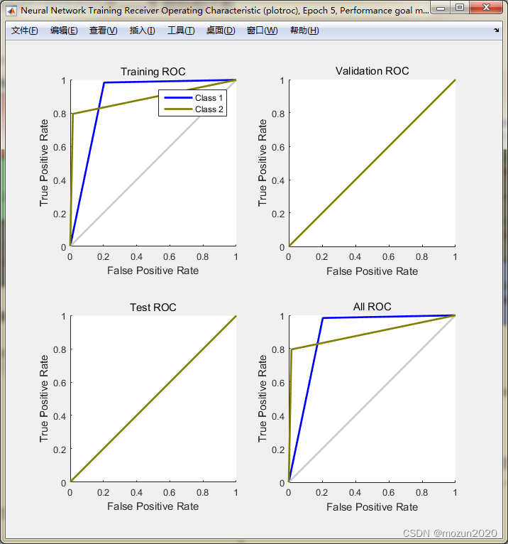
In turn, click Plots Medium Performance,Training State,Confusion,Receiver Operating Characteristic, The following figure can pop up ：




go back to MATLAB in , Open file view chapter26_bp.m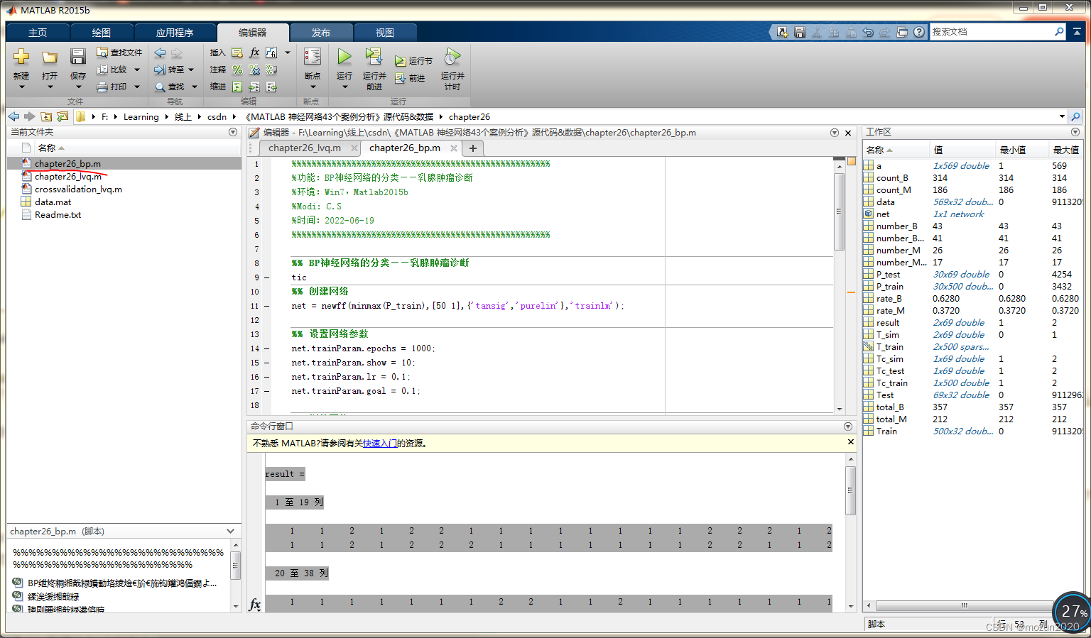

chapter26_bp.m Source code is as follows ：

%%%%%%%%%%%%%%%%%%%%%%%%%%%%%%%%%%%%%%%%%%%%%%%%%%%%
% function ：BP Classification of neural networks —— Breast tumor diagnosis 
% Environmental Science ：Win7,Matlab2015b
%Modi: C.S
% Time ：2022-06-19
%%%%%%%%%%%%%%%%%%%%%%%%%%%%%%%%%%%%%%%%%%%%%%%%%%%%

%% BP Classification of neural networks —— Breast tumor diagnosis 
tic
%%  Creating networks 
net = newff(minmax(P_train),[50 1],{
    'tansig','purelin'},'trainlm');

%%  Set network parameters 
net.trainParam.epochs = 1000;
net.trainParam.show = 10;
net.trainParam.lr = 0.1;
net.trainParam.goal = 0.1;

%%  Training network 
net = train(net,P_train,Tc_train);

%%  The simulation test 
T_sim = sim(net,P_test);
for i = 1:length(T_sim)
    if T_sim(i) <= 1.5
        T_sim(i) = 1;
    else
        T_sim(i) = 2;
    end
end
result = [T_sim;Tc_test]

number_B = length(find(Tc_test == 1));
number_M = length(find(Tc_test == 2));
number_B_sim = length(find(T_sim == 1 & Tc_test == 1));
number_M_sim = length(find(T_sim == 2 &Tc_test == 2));

disp([' Total number of cases ：' num2str(569)...
      '  Benign ：' num2str(total_B)...
      '  Malignant ：' num2str(total_M)]);
disp([' Total number of training set cases ：' num2str(500)...
      '  Benign ：' num2str(count_B)...
      '  Malignant ：' num2str(count_M)]);
disp([' Total number of cases in the test set ：' num2str(69)...
      '  Benign ：' num2str(number_B)...
      '  Malignant ：' num2str(number_M)]);
disp([' Benign breast tumor was diagnosed ：' num2str(number_B_sim)...
      '  Misdiagnosis ：' num2str(number_B - number_B_sim)...
      '  Diagnostic rate p1=' num2str(number_B_sim/number_B*100) '%']);
disp([' Malignant breast tumor was diagnosed ：' num2str(number_M_sim)...
      '  Misdiagnosis ：' num2str(number_M - number_M_sim)...
      '  Diagnostic rate p2=' num2str(number_M_sim/number_M*100) '%']);
  toc

Click on “ function ”, Start emulating , The output simulation results are as follows ：

result =

  1  to  19  Column 

     1     1     2     1     2     2     1     1     1     1     1     1     1     1     2     2     2     1     2
     1     1     2     1     2     2     2     1     1     1     1     1     1     1     2     2     1     1     2

  20  to  38  Column 

     1     1     1     1     1     1     1     2     2     1     1     2     1     1     1     1     1     1     1
     2     1     1     1     1     1     1     2     2     1     1     2     1     1     1     1     1     1     1

  39  to  57  Column 

     1     1     1     1     1     1     1     1     2     2     1     1     2     2     2     1     1     1     1
     1     2     2     2     2     2     1     1     2     2     2     1     2     2     1     1     1     1     1

  58  to  69  Column 

     1     1     1     2     2     2     1     1     1     1     2     1
     1     1     1     2     2     2     1     2     1     1     2     1

 Total number of cases ：569   Benign ：357   Malignant ：212
 Total number of training set cases ：500   Benign ：314   Malignant ：186
 Total number of cases in the test set ：69   Benign ：43   Malignant ：26
 Benign breast tumor was diagnosed ：41   Misdiagnosis ：2   Diagnostic rate p1=95.3488%
 Malignant breast tumor was diagnosed ：17   Misdiagnosis ：9   Diagnostic rate p2=65.3846%
 Time has passed  6.838382  second .
>> chapter26_bp

result =

  1  to  19  Column 

     1     1     2     1     2     2     2     1     1     1     1     1     1     1     2     2     1     2     2
     1     1     2     1     2     2     2     1     1     1     1     1     1     1     2     2     1     1     2

  20  to  38  Column 

     1     1     1     2     1     1     2     2     2     1     1     2     1     1     1     1     1     1     1
     2     1     1     1     1     1     1     2     2     1     1     2     1     1     1     1     1     1     1

  39  to  57  Column 

     1     2     2     2     2     2     2     1     1     2     2     2     2     2     2     2     1     1     1
     1     2     2     2     2     2     1     1     2     2     2     1     2     2     1     1     1     1     1

  58  to  69  Column 

     1     1     1     2     1     2     2     2     1     2     2     1
     1     1     1     2     2     2     1     2     1     1     2     1

 Total number of cases ：569   Benign ：357   Malignant ：212
 Total number of training set cases ：500   Benign ：314   Malignant ：186
 Total number of cases in the test set ：69   Benign ：43   Malignant ：26
 Benign breast tumor was diagnosed ：34   Misdiagnosis ：9   Diagnostic rate p1=79.0698%
 Malignant breast tumor was diagnosed ：23   Misdiagnosis ：3   Diagnostic rate p2=88.4615%
 Time has passed  2.954276  second .

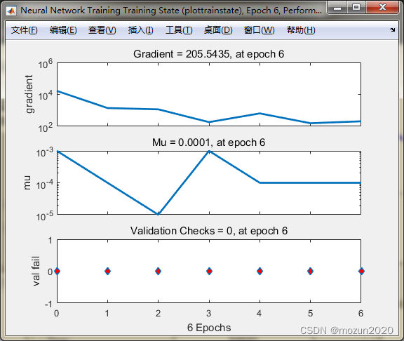
In turn, click Plots Medium Performance,Training State,Regression, The following figure can pop up ：

3. Summary

LVQ(Learning Vector Quantization) Neural network is Kohonen On 1989 In, a learning vector quantization network based on competitive network was proposed , Mainly used for classification . It belongs to the type of feedforward neural network , It has a wide range of applications in the field of pattern recognition and optimization .LVQ The neural network consists of three layers , Input layer 、 The hidden layer and the output layer , The network is fully connected between the input layer and the hidden layer , The hidden layer and the output layer are partially connected , Each output layer neuron is connected to a different group of hidden layer neurons . The connection weight between hidden layer and output layer neurons is fixed as 1. The weights of the connections between the neurons in the input layer and the hidden layer establish the components of the reference vector （ Assign a reference vector to each hidden neuron ）. In the process of network training , These weights are modified . Hidden layer neurons （ Also known as Kohnen Neuron ） And output neurons have binary output values . When an input mode is sent to the network , The implicit neuron whose reference vector is closest to the input mode wins the competition because of the excitation , Thus allowing it to produce a “1”, Other hidden layer neurons are forced to produce “0”. The output neuron connected to the hidden layer neuron group containing the winning neuron also emits “1”, Other output neurons all send out “0”. produce “1” The output neuron of gives the class of input pattern , thus it can be seen , Each output neuron is used to represent a different class .

This chapter will LVQ Neural networks and BP Comparative simulation of neural network in breast tumor diagnosis and prediction , It can be seen that in the prediction of benign and malignant ,LVQ Neural networks and BP Each neural network has its own advantages and disadvantages , The simulation of this example needs to run LVQ Get the corresponding data , Run again BP Conduct simulation . Interested in the content of this chapter or want to fully learn and understand , I suggest you study Chapter 26 of the book . Some of these knowledge points will be supplemented on the basis of their own understanding in the later stage , Welcome to study and exchange together .