当前位置:网站首页>Classification of traffic signs
Classification of traffic signs
2022-06-22 02:54:00 【-Small transparency-】
brief introduction
Traffic signs are one of the powerful tools to assist in judging and restraining drivers , And the traffic sign recognition system is also ADAS( Advanced driving AIDS ) One of the components of the scene , The system will enable the car to automatically recognize the traffic signs ahead and remind the driver . We may be able to look through the characteristics of traffic signs , Extract the part of the traffic sign from the image . How to identify the contents of the extracted traffic signs , This is what the machine learning model does .
1. Data integration
The original data sets are stored in their respective directories according to the names of traffic signs , And for machine learning models , Only training data and labels need to be transferred during training . therefore , We need to integrate the data to be trained .
Python3 file :DataIntegration.ipynb
import numpy as np
import os
import cv2 as cv
import tqdm
from tqdm import tqdm
# Complete the integration of data sets in this function , Function receive 1 Parameters , Data set path
def loadData(oriPath):
# Define the input image resolution of the model as 128 * 128 * 3
x = np.empty([0, 128, 128, 3])
# Usually, data labels are represented by numbers , So the defined label shape by [0] that will do .
y = np.empty([0])
# use os.listdir Function to traverse the list of data set types , Returns the names of all the files in this path
classNames = os.listdir(oriPath)
print(classNames)
# Traverse the list of data set types , Read data in each cycle
for i in range(len(classNames)):
if(classNames[i] != '.ipynb_checkpoints'):
# Get the names of all traffic sign images under the current label directory
labelPath = os.listdir(oriPath + '/' + classNames[i])
# Traverse the traffic sign image name array , The same goes for .ipynb_checkpoints The verdict of
for j in tqdm(range(len(labelPath))):
if(labelPath[j] != '.ipynb_checkpoints'):
# The relative path of combining the current traffic signs , And stored in imagePath variable
imageName = labelPath[j]
imagePath = oriPath + '/' + classNames[i] + '/' + imageName
# Read the image from the hard disk and store it in numpy Array
image = cv.imread(imagePath)
# The original BGR Three channel conversion to RGB Three channels
image = cv.cvtColor(image, cv.COLOR_BGR2RGB)
# Machine learning models require the same resolution of incoming data , By looking at the traffic sign image, you can find ,
# The image resolution of the original data is different
# Convert the resolution of the image to 128 * 128 * 3, This function can zoom in and out the image
image = cv.resize(image, (128, 128))
# Expand single image data by one dimension , Make it a size of 1 An array of images
image = np.expand_dims(image, axis = 0)
# Merge the extracted picture into the total picture variable , This function can be used to merge multiple shape Value , Such as images
x = np.concatenate((x, image), axis = 0)
# Merge the extracted tags into the total tag
y = np.append(y, i)
# Return data set x And tag sets y Value
return x, y# Yes Codelab/data The data sets in the catalog are integrated
x, y = loadData('data')
# Regularly stored data sets will affect model training , Therefore, the integrated data sets need to be randomly scrambled
permutation = np.random.permutation(y.shape[0])
x = x[permutation, :]
y = y[permutation]
# Split the dataset into 80% Training set and 20% Test set of .
testLength = int(x.shape[0]/100*(0.2*100))
xTest = x[0:testLength, :]
yTest = y[0:testLength]
xTrain = x[testLength:x.shape[0], :]
yTrain = y[testLength:y.shape[0]]
# Export datasets
np.save('xTrain.npy', xTrain)
np.save('yTrain.npy', yTrain)
np.save('xTest.npy', xTest)
np.save('yTest.npy', yTest)2. Data preprocessing
Python3 file :DataProcessing.ipynb
import tensorflow as tf
import tensorflow.keras as keras
import tensorflow.keras.layers as layers
import numpy as np
import matplotlib.pyplot as plt
from random import randint
import datetime
import cv2 as cv
%matplotlib inline
# Read the data set processed in the previous step
xTrain = np.load('xTrain.npy')
yTrain = np.load('yTrain.npy')
xTest = np.load('xTest.npy')
yTest = np.load('yTest.npy')# Copy the array corresponding to the label in the previous step , And named it labelSets
labelSets = ['limit40', 'limit80', 'parking', 'turnAround', 'walking']
numClasses = len(labelSets)Run the following code several times , View the sampling results . If the label name in the output corresponds to the figure below , Then the data set is read successfully
# In order to verify whether the data set is read correctly and whether the labels correspond accurately , Select in training set and test set respectively  1  Picture using  matplotlib  Display and use  OpenCV  Output to local .
index = randint(0, len(xTrain))
print(labelSets[int(yTrain[index])])

trainSingleImage = xTrain[index].astype(np.uint8)
plt.imshow(trainSingleImage)
plt.show()

trainSingleImage = cv.cvtColor(trainSingleImage, cv.COLOR_RGB2BGR)
cv.imwrite('test1.png', trainSingleImage)

print('----------------')

index = randint(0, len(xTest))
print(labelSets[int(yTest[index])])
testSingleImage = xTest[index].astype(np.uint8)
plt.imshow(testSingleImage)
plt.show()

testSingleImage = cv.cvtColor(testSingleImage, cv.COLOR_RGB2BGR)
cv.imwrite('test2.png', testSingleImage)
Usually , The value of each pixel of the image is in 0~255 Between , The upper and lower spans are large . If you use raw data directly , During training, it will be biased to pixels with higher values . therefore , In order to truly reflect the actual situation of the data , You need to preprocess the data .
# Divide the values of all pixels by  255  The way , Compress all pixel values to  0~1  Between
xTrain /= 255.0
xTest /= 255.0
The task of traffic sign recognition is a multi classification task , In multi category tasks , The tag values in the dataset need to be one-hot Operation to extend the eigenvector . That is to say, the label in the original data set 1, 2, 3, 4, 5 Use only one 1 And a number of 0 Eigenvector representation of
# Conduct one-hot code
yTrain = keras.utils.to_categorical(yTrain, numClasses)
yTest = keras.utils.to_categorical(yTest, numClasses)
# Output the converted training set and test set
print(xTrain[0])
print('-----')
print(yTrain[0])
print('-----')
print(xTest[0])
print('-----')
print(yTest[0])# Store the processed code locally
np.save('xTrainFinal.npy', xTrain)
np.save('yTrainFinal.npy', yTrain)
np.save('xTestFinal.npy', xTest)
np.save('yTestFinal.npy', yTest)3. structure CNN Classifier model
Python3 Of documents Training.ipynb
import tensorflow as tf
import tensorflow.keras as keras
import tensorflow.keras.layers as layers
import numpy as np
from random import randint
import datetime
import cv2 as cv
# Read the data set processed in the previous step
xTrain = np.load('xTrainFinal.npy')
yTrain = np.load('yTrainFinal.npy')
xTest = np.load('xTestFinal.npy')
yTest = np.load('yTestFinal.npy')# Use tf-keras Definition CNN Model
# When using this method to define the model, you only need to call the corresponding API Fill in the parameters of each layer of the model ,
#keras The training model layer will be automatically generated . The core of this model is 3 Layer convolution pooling combination ,1 Layer flattening and 2 Layer full connection .
model = keras.Sequential()
model.add(layers.Convolution2D(16, (3, 3),
padding='same',
input_shape=xTrain.shape[1:], activation='relu'))
model.add(layers.MaxPooling2D(pool_size=(2, 2)))
model.add(layers.Convolution2D(32, (3, 3), padding='same', activation= 'relu'))
model.add(layers.MaxPooling2D(pool_size=(2, 2)))
model.add(layers.Convolution2D(64, (3, 3), padding='same', activation= 'relu'))
model.add(layers.MaxPooling2D(pool_size =(2,2)))
model.add(layers.Flatten())
model.add(layers.Dense(128, activation='relu', kernel_regularizer=keras.regularizers.l2(0.001)))
model.add(keras.layers.Dropout(0.75))
model.add(layers.Dense(5, activation='softmax'))# Define the optimizer and initialize tf-keras Model
# Set the loss function to “ Multi class logarithmic loss function ”
# The performance evaluation function is to calculate the multi classification accuracy , That is, whether the subscript value of the maximum value is the same as the label value .
adam = keras.optimizers.Adam()
model.compile(loss='categorical_crossentropy',
optimizer=adam,
metrics=['categorical_accuracy'])
print(model.summary())# Display the training results visually
# We use Tensorboard Callback .Tensorboard The loss value in the model training process , Evaluation value and other important parameter records , Help optimize the model ,
# Through some configuration ,Tensorboard It can even complete the function of data set evaluation preview .
logDir="logs/" + datetime.datetime.now().strftime("%Y%m%d-%H%M%S")
tensorboardCallback = tf.keras.callbacks.TensorBoard(log_dir=logDir, histogram_freq=1)4. Train and evaluate the model
# Use  TensorFlow 2.0  in  tf.data  The new feature of parallelization strategy
trainDataTensor = tf.constant(xTrain)
trainLabelTensor = tf.constant(yTrain)

evalDataTensor = tf.constant(xTest)
evalLabelTensor = tf.constant(yTest)
# Use tf.data Of from_tensor_slices establish tf.data, This function needs to pass in a length of 2 tuples ,
# Represent training data respectively Tensor and Training tags Tensor, Function returns the generated tf.data Variable
trainDatasets = tf.data.Dataset.from_tensor_slices((trainDataTensor, trainLabelTensor))
evalDatasets = tf.data.Dataset.from_tensor_slices((evalDataTensor, evalLabelTensor))# Set up tf.data Of batch The size is 64, And use prefetch function .
trainDatasets = trainDatasets.batch(32)
trainDatasets = trainDatasets.prefetch(tf.data.experimental.AUTOTUNE)
evalDatasets = evalDatasets.batch(32)
evalDatasets = evalDatasets.prefetch(tf.data.experimental.AUTOTUNE)#fit Function execution training , This function supports passing in tf.data As training set and test set
model.fit(x = trainDatasets, validation_data = evalDatasets, epochs = 10, callbacks=[tensorboardCallback])
# meanwhile , Add... To the training callback function Tensorboard Recording function Execution procedure 4, You can see the training process .
Wait until the training is over , In the directory tree on the left logs Catalog , In this directory, there are Tensorboard file .
Double click in the left sidebar to enter logs After the directory , choice Tensorboard You can view it
# Store the trained model locally
model.save('model.h5')
source -- AI Explorer
边栏推荐
- xpm_ memory_ A complete example of using the tdpram primitive
- June25,2022 PMP Exam clearance manual-5
- 如何选择合适的 Neo4j 版本(2022版)
- Horizontal comparison of domestic API management platforms, which one is stronger?
- Day14QProgressBar2021-10-17
- C ++ Primer 第2章 变量和基本类型 总结
- 【一起上水硕系列】Day Two
- 使用开源软件攒一个企业级图数据平台解决方案
- C2-qt serial port debugging assistant 2021.10.21
- JVM makes wheels
猜你喜欢
xpm_memory_tdpram原语的完整使用实例

PMP备考相关敏捷知识

【2. 归并排序】

How to select the appropriate version of neo4j (version 2022)

Zhixiang Jintai rushes to the scientific innovation board: the annual revenue is 39.19 million, the loss is more than 300million, and the proposed fund-raising is 4billion

The brand, products and services are working together. What will Dongfeng Nissan do next?
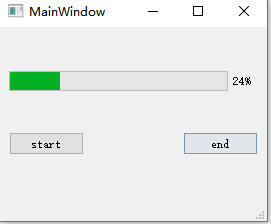
Day14QProgressBar2021-10-17
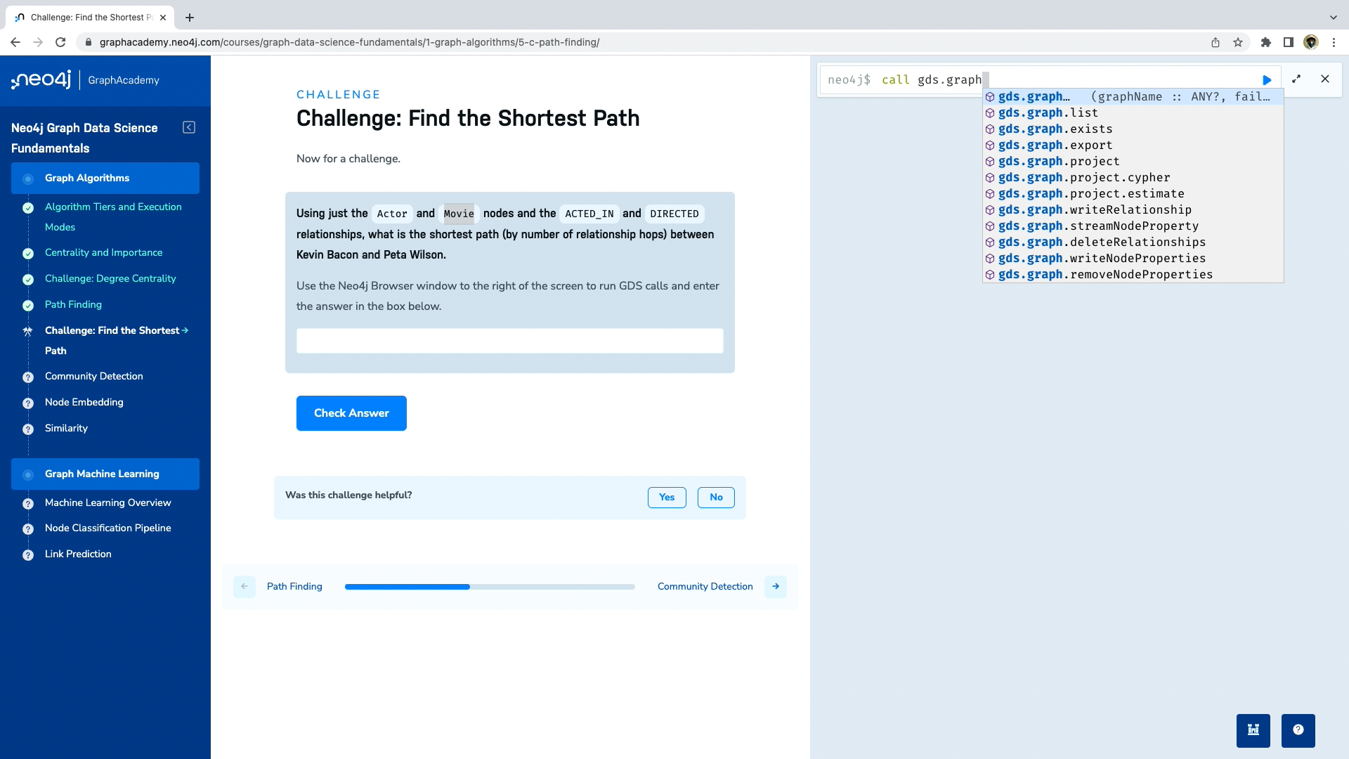
Graphacademy course explanation: Fundamentals of neo4j graph data science
![[go language] we should learn the go language in this way ~ a comprehensive learning tutorial on the whole network](/img/91/324d04dee0a191725a0b8751375005.jpg)
[go language] we should learn the go language in this way ~ a comprehensive learning tutorial on the whole network

Official release of ideal L9: retail price of 459800 yuan will be delivered before the end of August
随机推荐
discuz! Bug in the VIP plug-in of the forum repair station help network: when the VIP member expires and the permanent member is re opened, the user group does not switch to the permanent member group
使用 Neo4j 沙箱学习 Neo4j 图数据科学 GDS
Force buckle 461 Hamming distance
Neo4j 智能供应链应用源代码简析
Parallel search DSU
【9. 子矩阵和】
Neo4j 技能树正式发布,助你轻松掌握Neo4j图数据库
Using JMeter for web side automated testing
PMP pre exam guide on June 25, you need to do these well
C2-qt serial port debugging assistant 2021.10.21
tag动态规划-刷题预备知识-1.动态规划五部曲解题法 + lt.509. 斐波那契数/ 剑指Offer 10.I + lt.70. 爬楼梯彻底解惑 + 面试真题扩展
Implementation principle and application practice of Flink CDC mongodb connector
import和require在浏览器和node环境下的实现差异
Day14QProgressBar2021-10-17
B-Tree
【4. 高精度加法】
Sword finger offer 12 Path in matrix
[Shangshui Shuo series] day two
[2. merge sort]
Dynamically load assetdatabase of assets