(CVPR 2020) Learning Object Bounding Boxes for 3D Instance Segmentation on Point Clouds

Abstract

We put forward a new 、 A general framework that is conceptually simple , Used in 3D Instance segmentation on the point cloud . Our approach is called 3D-BoNet, Follow the multilayer perceptron at each point (MLP) Simple design concept . The framework directly regresses all instances in the point cloud 3D Bounding box , Predict the point level of each instance at the same time （point-level） Mask . It consists of a backbone network and two parallel network branches , be used for 1） Bounding box regression and 2） Dot mask prediction .3D-BoNet It's a single stage 、anchor-free And end-to-end trainable . Besides , Its computational efficiency is very high , Because it is different from the existing methods , It does not require any post-processing steps , For example, non maximum suppression 、 Feature sampling 、 Clustering or voting . A lot of experiments show that , Our approach goes beyond ScanNet and S3DIS Existing work on datasets , At the same time, the computational efficiency is improved by about 10 times . Comprehensive ablation studies have demonstrated the effectiveness of our design .

1 Introduction

Make the machine understand 3D The scene is autopilot 、 Basic prerequisites for augmented reality and robotics . Point cloud, etc 3D The core problem of geometric data includes semantic segmentation 、 Object detection and instance segmentation . In these questions , Instance segmentation has only begun to be solved in the literature . The main obstacle is that the point cloud is essentially disordered 、 Unstructured and uneven . The widely used convolutional neural network needs to 3D Voxelization of point cloud , This results in high computing and memory costs .

The first direct processing 3D The neural algorithm for instance segmentation is SGPN [50], It uses similarity matrix learning to group the features of each point . Similarly ,ASIS [51]、JSIS3D[34]、MASC[30]、3D-BEVIS[8] and [28] Group the same features per point pipeline Apply to segmentation 3D example . Mo Et al. Expressed the instance segmentation as PartNet[32] Point by point feature classification in . However , these proposal-free The learning fragment of method does not have high objectiveness , Because they do not explicitly detect the target boundary . Besides , They inevitably require post-processing steps , For example, mean shift clustering [6] To get the final instance tag , This is computationally onerous . the other one pipeline Is based on proposal Of 3D-SIS[15] and GSPN[58], They usually rely on two-stage training and expensive non maximum inhibition to trim dense targets proposal.

In this paper , We propose an elegant 、 Efficient and novel 3D Instance segmentation framework , By using efficient MLPs Single forward phase of , Loose but unique detection of objects , Then a simple point level binary classifier is used to segment each instance accurately . So , We introduce a new bounding box prediction module and a series of well-designed loss functions to directly learn the target boundary . Our framework is based on proposal and proposal-free There is a big difference in the way , Because we can effectively segment all instances with high goals , But don't rely on expensive and dense targets proposal. Our code and data are available in https://github.com/Yang7879/3D-BoNet get .

chart 1： stay 3D Point cloud for instance segmentation 3D-BoNet frame .

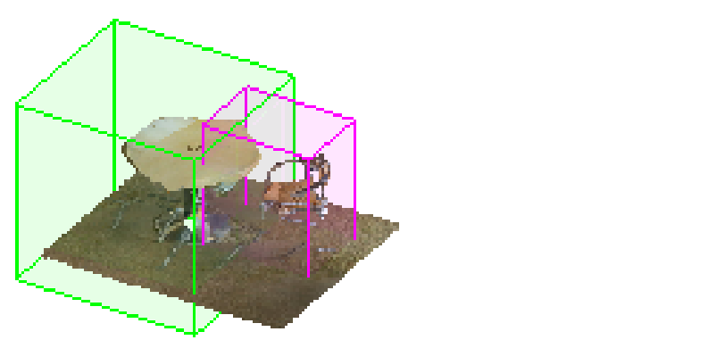
Bounding box prediction branch is the core of our framework . This branch is intended for single forward Each instance in the phase predicts a unique 、 Directionless rectangular bounding box , Instead of relying on predefined spaces anchors Or area proposal The Internet [39]. Pictured 2 Shown , We think it is a rough drawing for the example 3D Bounding boxes are relatively realizable , Because the input point cloud explicitly contains 3D Geometric information , It is very useful before dealing with point level instance segmentation , Because a reasonable bounding box can ensure the high goal of the learning segment . However , The learning example box covers key issues ：1） The total number of instances is variable , From 1 To many ,2） There is no fixed order for all instances . These problems pose great challenges to the correct optimization of the network , Because there is no information that can directly link the prediction box to ground truth Tags are linked to monitor the network . however , We showed how to solve these problems gracefully . This box prediction branch simply takes the global eigenvector as input , And directly output a large number of fixed number of bounding boxes and confidence scores . These scores are used to indicate whether the box contains valid instances . To monitor the network , We design a novel bounding box correlation layer , Then there is a multi standard loss function . Give a group ground-truth example , We need to determine which prediction box is best for them . We express this association process as an optimal assignment problem with existing solvers . After the box is best associated , Our multi criteria loss function not only minimizes the Euclidean distance of the pairing box , And it maximizes the coverage of effective points in the prediction frame .

chart 2： Rough example box .

The predicted box is then input into the subsequent point mask prediction branch along with the point and global features , To predict a dot level binary mask for each instance . The purpose of this branch is to classify whether each point in the bounding box belongs to a valid instance or background . Suppose the estimated instance box is quite good , It is possible to obtain an accurate dot mask , Because this branch simply rejects points that do not belong to the detected instance . Random guessing may lead to 50% Amendment .

Overall speaking , Our framework is similar to all existing ones in three aspects 3D Instance segmentation methods are different .1） And proposal-free pipeline comparison , Our approach is through explicit learning 3D Target boundary is used to segment high target instances . 2） And widely used based on proposal Compared with , Our framework doesn't need to be expensive and dense proposal.3） Our framework is very efficient , Because instance level （instance-level） The mask is in a single forward （single-forward） Learning through transmission , No post-processing steps are required . Our main contribution is ：

• We propose a method in 3D A new framework for instance segmentation on point cloud . The framework is one-stage 、anchor-free And end-to-end trainable , No post-processing steps are required .

• We design a novel bounding box correlation layer , Then there is a multi standard loss function to monitor the prediction branch of the box .

• We showed that it was right baselines Significant improvements in , Extensive ablation studies have provided an intuitive basis for our design choices .

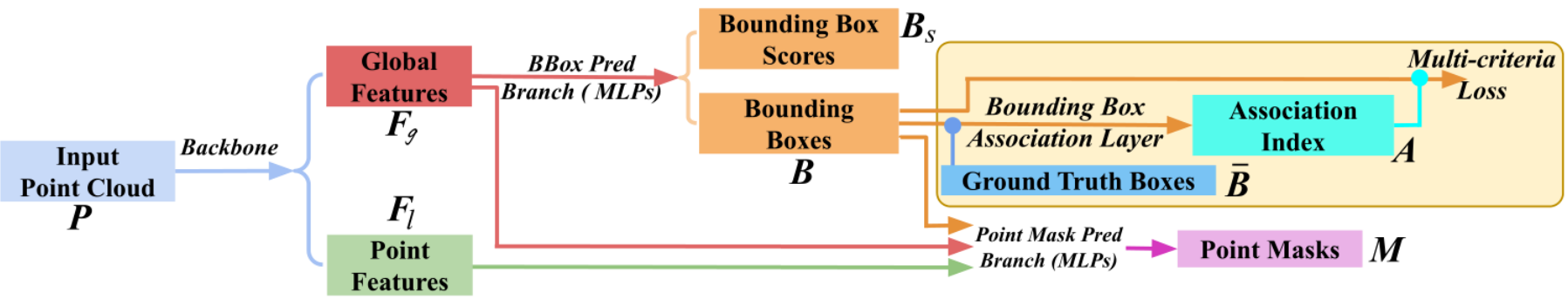
chart 3：3D-BoNet The general workflow of the framework .

2 3D-BoNet

2.1 Overview

Pictured 3 Shown , Our framework consists of two branches at the top of the backbone network . Given a common $N$ Input point cloud of points $\mathbf{P}$, namely $\mathbf{P}\in {\mathbb{R}}^{N\times k_0}$, among $k_0$ Is the position of each point $\{x,y,z\}$ And color $\{r,g,b\}$ Number of equal channels , Backbone network extracts local features of points , Write it down as ${\mathbf{F}}_l\in {\mathbb{R}}^{N\times k}$, Aggregate a global point cloud feature vector , Write it down as ${\mathbf{F}}_g\in {\mathbb{R}}^{1\times k}$, among $k$ Is the length of the eigenvector .

The bounding box prediction branch simply converts the global eigenvector ${\mathbf{F}}_g$ As input , And directly regress a set of predefined and fixed bounding boxes , Write it down as $\mathbf{B}$, And the corresponding box fraction , Write it down as ${\mathbf{B}}_s$. We use ground truth Bounding box information to monitor this branch . During training , The predicted bounding box $\mathbf{B}$ and ground truth Box is associated with the input box . This layer is designed to automatically match the unique and most similar prediction bounding box with each ground truth Box is associated with . The output of the association layer is the association index $A$ A list of . Index reorganize forecast box , Make each ground truth Box is paired with a unique prediction box , For subsequent loss calculation . Before calculating the loss , The predicted bounding box scores are also reordered accordingly . Then input the reordered prediction boundary box into the multi standard loss function . Basically , This loss function is not only intended to minimize each ground truth Euclidean distance between the frame and the related prediction frame , It also maximizes the coverage of effective points in each prediction frame . Please note that , Both the bounding box correlation layer and the multi criteria loss function are designed only for network training . They are discarded during testing . Final , This branch can directly predict the correct bounding box and box score of each instance .

To predict the of each instance point-level Binary mask , Each prediction box together with the previous local and global features , namely ${\mathbf{F}}_l$ and ${\mathbf{F}}_g$, Is further fed into the dot mask prediction branch . This network branch is shared by all instances of different classes , So it is very light and compact . This category independent approach essentially allows for general segmentation across invisible categories .

2.2 Bounding Box Prediction

Bounding box coding ： In the existing target detection network , The bounding box usually consists of the center position and the length of three dimensions [3] Or the corresponding residual [60] And direction . contrary , For the sake of simplicity , We only pass through two min-max Vertex parameterized rectangular bounding box ：

$$\left\{\left[\begin{array}{ll}{x}_{\min }{y}_{\min }& z_{\min }\end{array}\right],\left[\begin{array}{lll}{x}_{\max }& y_{\max }& z_{\max }\end{array}\right]\right\}$$

Nerve layer ： Pictured 4 Shown , Global eigenvector ${\mathbf{F}}_g$ Feed... Through two fully connected layers , among Leaky ReLU As a nonlinear activation function . Then there are two other parallel fully connected layers . One layer outputs one 6H Dimension vector , Then reshape it to $H\times 2\times 3$ tensor . $H$ Is a predefined and fixed number of bounding boxes , The whole network is expected to have the largest prediction . Another layer outputs a $H$ Dimension vector , Heel sigmoid Function to represent the bounding box fraction . The higher the score , The more likely the prediction box contains instances , So this box is more effective .

Bounding box associative layer ： Given the previously predicted $H$ A bounding box , namely $B\in {\mathbb{R}}^{H\times 2\times 3}$, Use as $\overline{\mathbf{B}}\in {\mathbb{R}}^{T\times 2\times 3}$ Of ground truth Box to monitor the network , Because there is no predefined in our framework anchors Each prediction box can be traced back to the corresponding ground truth box . Besides , For each input point cloud $\mathbf{P}$,ground truth box $T$ The number of is different , And usually with a predefined number $H$ Different , Although we can safely assume a predefined number of all input point clouds $H\ge T$. Besides , Prediction box or ground truth Boxes have no box order .

chart 4： The architecture of the bounding box regression branch . Before calculating the multi standard loss , Predicted $H$ Boxes and $T$ individual ground truth Box best Association .

Optimal correlation formula ： In order to $\mathbf{B}$ The unique prediction bounding box in $\overline{\mathbf{B}}$ Each ground truth Box is associated with , We express this correlation process as an optimal allocation problem . Formally , Give Way $A$ Is a Boolean incidence matrix , among ${\mathbf{A}}_{i,j}=1$, If and only if $i$ A prediction box is assigned to the $j$ individual ground truth box . $A$ It is also called correlation index in this paper . Make $C$ For the connection cost matrix , among ${\mathbf{C}}_{i,j}$ It means that the $i$ The prediction box is assigned to the $j$ individual ground truth Framed cost. Basically ,cost ${\mathbf{C}}_{i,j}$ Indicates the similarity between two boxes ;cost The lower the , The more similar the two boxes are . therefore , The problem of bounding box association is to find the total cost Minimum optimal allocation matrix $A$：

$$\mathbf{A}=\underset{\mathbf{A}}{\mathrm{argmin}}\sum _{i=1}^H\sum _{j=1}^T{\mathbf{C}}_{i,j}{\mathbf{A}}_{i,j}\text{ subject to }\sum _{i=1}^H{\mathbf{A}}_{i,j}=1,\sum _{j=1}^T{\mathbf{A}}_{i,j}\le 1,j\in \{1..T\},i\in \{1..H\}(1)$$

In order to solve the above optimal correlation problem , The existing Hungarian Algorithm [20; 21] application . Incidence matrix calculation ： In order to evaluate the $i$ Prediction box and $j$ individual ground truth Similarity between , A simple and intuitive criterion is two pairs of minima - The Euclidean distance between the largest vertices . However , It's not the best . Basically , We want the prediction box to contain as many valid points as possible . Pictured 5 Shown , The input point cloud is usually sparse , And in 3D Uneven distribution in space . For the same ground truth box #0（ Blue ）, Candidate box #2（ Red ） Considered to be better than the candidate box #1（ black ） It's much better , Because the box #2 There are more effective points and #0 overlap . therefore , In the calculation cost matrix $C$ when , The coverage of effective points shall be included . In this paper , We consider the following three criteria ：

chart 5： Sparse input point cloud .

Algorithm 1 An algorithm for calculating the probability of points in the prediction frame .$H$ Yes prediction bounding box $\mathbf{B}$ The number of ,$N$ It's point cloud $\mathbf{P}$ Points in ,${\theta }_1$ and ${\theta }_2$ Is a hyperparameter of numerical stability . We use... In all our implementations ${\theta }_1=100$, ${\theta }_2=20$.

The above two cycles are for illustration only . They are easily replaced by standard and efficient matrix operations .

(1) Euclidean distance between vertices . Formally , The first $i$ A prediction box ${\mathbf{B}}_i$ And the $j$ individual ground truth box ${\overline{\mathbf{B}}}_j$ The cost between is calculated as follows ：

$${\mathbf{C}}_{i,j}^{ed}=\frac{1}{6}\sum {\left({\mathbf{B}}_i-{\overline{\mathbf{B}}}_j\right)}^2(1)$$

(2) Point on the soft Intersection-over-Union. Given input point cloud $\mathbf{P}$ And the $j$ individual ground truth Instance box ${\overline{\mathbf{B}}}_j$, You can get one directly hard-binary vector ${\overline{\mathbf{q}}}_j\in {\mathbb{R}}^N$ To indicate whether each point is in the box , among ’1’ It means that the point is inside , It's outside “0”. However , For the same input point cloud $\mathbf{P}$ Specific section of $i$ A prediction box , Due to the discrete operation , Get similar directly hard-binary The vector will cause the frame to be nondifferentiable . therefore , We introduce a differentiable but simple algorithm 1 To get a similar but soft-binary vector ${\mathbf{q}}_i$, be called point-in-pred-box-probability, All of these values are in $(0,1)$ Within the scope of . The deeper the corresponding point is in the box , The higher the value . The farther the point , The smaller the value. . Formally , The first $i$ Prediction box and $j$ individual ground truth Soft cross joint between frames （sIoU）cost The definition is as follows ：

$${\mathbf{C}}_{i,j}^{sIoU}=\frac{-{\sum }_{n=1}^N\left(q_i^n\ast {\bar{q}}_j^n\right)}{{\sum }_{n=1}^N{q}_i^n+{\sum }_{n=1}^N{\bar{q}}_j^n-{\sum }_{n=1}^N\left(q_i^n\ast {\bar{q}}_j^n\right)}(3)$$
among $q_i^n$ and ${\bar{q}}_j^n$ yes ${\mathbf{q}}_i$ and ${\overline{\mathbf{q}}}_j$ Of the n It's worth .

(3) Cross entropy fraction . Besides , We also considered ${\mathbf{q}}_i$ and ${\overline{\mathbf{q}}}_j$ The cross entropy score between . And prefer tighter frames sIoU cost Different , This score represents the confidence that the predicted bounding box can contain as many effective points as possible . It prefers larger and more inclusive boxes , And formally defined as ：

$${\mathbf{C}}_{i,j}^{ces}=-\frac{1}{N}\sum _{n=1}^N\left[{\bar{q}}_j^n\log q_i^n+\left(1-{\bar{q}}_j^n\right)\log \left(1-q_i^n\right)\right](4)$$

Overall speaking , standard (1) The geometric boundary of the learning frame is guaranteed , standard (2)(3) Maximize the coverage of effective points and overcome the non-uniformity , Pictured 5 Shown . The first $i$ Prediction box and $j$ individual ground truth The box is defined as ：
$${\mathbf{C}}_{i,j}={\mathbf{C}}_{i,j}^{ed}+{\mathbf{C}}_{i,j}^{sIoU}+{\mathbf{C}}_{i,j}^{ces}(5)$$

The loss function follows the bounding box correlation layer , Prediction box $\mathbf{B}$ And fractions ${\mathbf{B}}_s$ All use associated indexes $A$ reorder , Make the first prediction $T$ Boxes and scores with $T$ individual ground truth Boxes are well matched .

Multi-criteria Loss for Box Prediction： The former correlation layer is based on the minimum cost （cost） For each ground truth Box find the most similar prediction box , Include ：1） Vertex Euclidean distance ,2） Point on sIoU cost （cost）, as well as 3） Cross entropy score . therefore , The loss function of the bounding box prediction is naturally designed to always minimize these costs （cost）. Its formal definition is as follows ：

$${\ell }_{bbox}=\frac{1}{T}\sum _{t=1}^T\left({\mathbf{C}}_{t,t}^{ed}+{\mathbf{C}}_{t,t}^{sIoU}+{\mathbf{C}}_{t,t}^{ces}\right)(6)$$

among ${\mathbf{C}}_{t,t}^{ed},{\mathbf{C}}_{t,t}^{sIoU}$ and ${\mathbf{C}}_{t,t}^{ces}$ It's No $t$ Cost of pairing boxes . Please note that , We only minimized T A pair of boxes cost; remainder H - T Forecast boxes ignored , Because they have no corresponding ground truth. therefore , This box predicts subbranches and H Is independent of the predefined value of . Here comes a question . because H - T Negative predictions go unpunished , Therefore, the network may predict multiple similar boxes for a single instance . Fortunately, , The loss function of parallel box fraction prediction can alleviate this problem .

The loss of box score prediction ： The prediction box score is intended to indicate the effectiveness of the corresponding prediction box . Indexed by association $A$ After reordering , front $T$ Scores ground truth The scores are “1”, The rest are invalid H-T The score is “0”. We use cross entropy loss for this binary classification task ：

$${\ell }_{bbs}=-\frac{1}{H}\left[\sum _{t=1}^T\log {\mathbf{B}}_s^t+\sum _{t=T+1}^H\log \left(1-{\mathbf{B}}_s^t\right)\right](7)$$

among ${\mathbf{B}}_s^t$ It is the... After association t A prediction score . Basically , This loss function rewards the bounding box for correct prediction , At the same time, it implicitly punishes the case that a single instance returns to multiple similar boxes .

2.3 Point Mask Prediction

Given the bounding box of the forecast $B$、 Point characteristics of learning ${\mathbf{F}}_l$ And global characteristics ${\mathbf{F}}_g$, The dot mask prediction branch processes each bounding box separately using a shared neural layer .

surface 1：ScanNet(v2) The benchmark （ Hide test sets ） Instance segmentation results on . The measure is IoU The threshold for 0.5 Of AP(%). On 2019 year 6 month 2 A visit to .

Nerve layer ： Pictured 6 Shown , Both the point and global features are compressed into 256 Dimension vector , Then connect and further compress to 128 Dimensional mixed point features ${\tilde{\mathbf{F}}}_l$. For the first $i$ Predicted bounding boxes ${\mathbf{B}}_i$, The estimated vertices and scores are connected with the features ${\tilde{\mathbf{F}}}_l$ The fusion , Generate frame aware features ${\hat{\mathbf{F}}}_l$. These features are then fed through the shared layer , forecast point-level Binary mask , Expressed as ${\mathbf{M}}_i$. We use sigmoid As the last activation function . It is similar to RoIAlign comparison , This simple frame fusion method is very effective in computation [58; 15; 13] This involves expensive point feature sampling and alignment .

Loss function ： According to the previous association index $\mathbf{A}$, Predicted instance mask $M$ And ground truth Masks are similarly associated with . Due to the imbalance of instance and background points , We use focus loss with default super parameters [29] Instead of standard cross entropy loss to optimize this branch . Only effective $T$ Pairing masks for loss function ${\ell }_{pmask}$.

chart 6： The architecture of the dot mask prediction branch . Point features are fused with each bounding box and fraction , Then predict one for each instance point-level Binary mask .

2.4 End-to-End Implementation

Although our framework is not limited to any point cloud network , But we use PointNet++[38] As a backbone for learning local and global features . meanwhile , Implemented another separate branch , To use standard softmax Cross entropy loss function ${\ell }_{\text{sem }}$ To learn every bit of semantics . The architecture of the trunk and semantic branches is similar to [50] The same as used in . Given an input point cloud $\mathbf{P}$, The above three branches are linked , And use a single combination of multi task losses for end-to-end training ：

$${\ell }_{\text{all }}={\ell }_{\text{sem }}+{\ell }_{bbox}+{\ell }_{bbs}+{\ell }_{\text{pmask }}(8)$$

We use Adam solver [18] And its default super parameters . The initial learning rate is set to $5e^{-4}$, Then each 20 individual epoch Divide 2. The whole network starts from scratch Titan X GPU Training on . We used the same settings for all experiments , This ensures the repeatability of our framework .

3 Experiments

3.1 Evaluation on ScanNet Benchmark

We started with ScanNet(v2) 3D Semantic instance segmentation benchmark [7] To evaluate our methods on the Internet . And SGPN[50] similar , We divide the original input point cloud into $1m\times 1m$ Block for training , Test with all points at the same time , And then use BlockMerging Algorithm [50] Assemble the block into a complete 3D scene . In our experiment , We observed that based on vanilla PointNet++ The performance of the semantic prediction sub branch is limited , Unable to provide satisfactory semantics . Due to the flexibility of our framework , So we can easily train a parallel SCN The Internet [11] For our 3D-BoNet The prediction instance estimates more accurate semantic labels per point .IoU The threshold for 0.5 The average accuracy of (AP) Used as an evaluation index .

We are with the table 1 in 18 The leading methods of target categories are compared . especially ,SGPN[50]、3D-BEVIS[8]、MASC[30] and [28] It is a method based on point feature clustering ;RPointNet[58] Learning to generate intensive goals proposals, Then point level segmentation ;3D-SIS[15] It's based on proposal Methods , Use point clouds and color images as input .PanopticFusion[33] Learn to pass Mask-RCNN[13] In more than one 2D Segmentation instance on image , And then use SLAM The system reprojects back to 3D Space . Our approach goes beyond them using only point clouds . It is worth noting that , Our framework performs relatively well in all categories , Instead of preferring specific classes , This proves the superiority of our framework .

chart 7： This shows that one contains hundreds of targets （ For example, chair 、 Table ） The lecture room , The challenge of instance segmentation is highlighted . Different colors represent different instances . The same instance may have different colors . Our framework predicts instance labels more accurately than other frameworks .

3.2 Evaluation on S3DIS Dataset

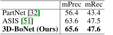
We further evaluated our framework in S3DIS[1] Semantic instance segmentation on , This includes coming from 6 A large area 271 A room 3D Full scan . Our data preprocessing and experimental setup strictly follow PointNet[37]、SGPN[50]、ASIS[51] and JSIS3D[34]. In our experiment ,$H$ Set to 24, We followed 6 Multiple evaluation [1; 51].

We and ASIS[51]、S3DIS The latest technology and PartNet baseline[32] Compare . For a fair comparison , We use the same as in our framework PointNet++ The trunk and other settings are carefully trained PartNet baseline. To evaluate , Reported IoU The threshold for 0.5 The average precision of classical indexes (mPrec) And the average recall rate (mRec). Please note that , For our methods and PartNet The baseline , Let's use the same one BlockMerging Algorithm [50] To merge instances from different blocks . The final score is a total of 13 Average of categories . surface 2 Shows mPrec/mRec fraction , chart 7 The qualitative results are shown . Our approach goes far beyond PartNet baseline[32], And better than ASIS[51], But not significantly , Mainly because of our semantic prediction branch （ be based on vanilla PointNet++） Not as good as ASIS, The latter closely integrates semantics and instance features to achieve mutual optimization . We take feature fusion as our future exploration .

surface 2：S3DIS The result of instance segmentation on dataset .

3.3 Ablation Study

To evaluate the effectiveness of each component of our framework , We are S3DIS The largest area of the dataset 5 On the 6 Group ablation experiment .

(1)Remove Box Score Prediction Sub-branch. Basically , The box fraction is used as the index and regularizer of effective bounding box prediction . After deleting it , We use the following methods to train the network ：

$${\ell }_{ab1}={\ell }_{sem}+{\ell }_{bbox}+{\ell }_{pmask}$$

first , Multi criteria loss function is Euclidean distance 、soft IoU A simple unweighted combination of cost and cross entropy scores . However , This may not be optimal , Because the density of the input point cloud is usually inconsistent , And tend to choose different criteria . The ablative boundary box loss function is 3 Group experiment .

surface 3：S3DIS Area 5 Segmentation results of all ablation experiments on the .

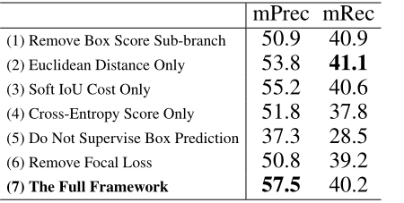
(2)-(4) Use a single standard . There is only one criterion for frame correlation and loss ${\ell }_{bbox}$.

$${\ell }_{ab2}={\ell }_{sem}+\frac{1}{T}\sum _{t=1}^T{\mathbf{C}}_{t,t}^{ed}+{\ell }_{bbs}+{\ell }_{pmask}\dots {\ell }_{ab4}={\ell }_{sem}+\frac{1}{T}\sum _{t=1}^T{\mathbf{C}}_{t,t}^{ces}+{\ell }_{bbs}+{\ell }_{pmask}$$

(5) Unsupervised box predictions . The prediction box is still associated according to three criteria , But we removed the box supervision signal . The framework has been trained as follows ：

$${\ell }_{ab5}={\ell }_{sem}+{\ell }_{bbs}+{\ell }_{pmask}$$

(6) Remove the dot mask prediction Focal Loss. In the dot mask prediction Branch , Replace the focus loss with the standard cross entropy loss for comparison .

analysis . surface 3 The scores of ablation experiments are shown . (1) box score Sub branches are really good for overall instance partitioning performance , Because it tends to punish repetition box forecast .(2) Compared with Euclidean distance and cross entropy score , Because of our differentiable algorithm 1, Frame related and supervised sIoU Costs tend to be better . Since three separate standards prefer different types of point structures , So three simple combinations on a particular dataset , Standards may not always be optimal .(3) If there is no monitoring of box predictions , Performance will degrade significantly , The main reason is that the network cannot infer a satisfactory instance 3D The border , And the quality of the prediction dot mask decreases accordingly .(4) And focal loss comparison , Due to the imbalance of instance and background points , The effect of standard cross entropy loss on point mask prediction is poor .

3.4 Computation Analysis

(1) For the method based on point feature clustering , Include SGPN[50]、ASIS[51]、JSIS3D[34]、3D-BEVIS[8]、MASC[30] and [28], The computational complexity of the post clustering algorithm, for example Mean Shift[6] Tend to $\mathcal{O}\left(T{N}^2\right)$, among $T$ Is the number of instances ,$N$ Is to enter the number of points .(2) For including GSPN[58]、3D-SIS[15] and PanopticFusion[33] Based on the intensive proposal Methods , Areas are usually required proposal Network and non maximum suppression to generate and prune dense proposal, It's computationally expensive [33]. (3)PartNet baseline[32] And our 3D-BoNet Both have similar effective computational complexity $\mathcal{O}(N)$. Based on experience , our 3D-BoNet It takes about 20 ms GPU Time to deal with 4k spot , and (1)(2) Most of the methods in need of more than 200 ms GPU/CPU Time to process the same number of points .

4 Related Work

In order to learn from 3D Feature extraction from point cloud , Traditional methods usually make features manually [5; 42]. Recently, learning based methods mainly include voxel based methods [42; 46; 41; 23; 40; 11; 4] And point based solutions [37; 19; 14; 16; 45].

Semantic Segmentation PointNet[37] It shows the leading results of classification and semantic segmentation , But it doesn't capture context features . To solve this problem , Many ways [38; 57; 43; 31; 55; 49; 26; 17] Recently proposed . Another pipeline is based on convolution kernel [55; 27; 47]. Basically , Most of these methods can be used as our backbone network , And with our 3D-BoNet Parallel training to learn each point of semantics .

Object Detection stay 3D The common method of detecting objects in point cloud is to project points to 2D Return to the bounding box on the image [25; 48; 3; 56; 59; 53]. Through fusion [3] Medium RGB Images , The detection performance is further improved RGB Images [3;54;36;52].. Point clouds can also be divided into voxels for target detection [9; 24; 60]. However , Most of these methods rely on predefined anchors and two-stage areas proposal The Internet [39]. stay 3D Extending them over point clouds is inefficient . Don't rely on anchors Under the circumstances , Current PointRCNN[44] Learn to detect through the front scenic spot segmentation , and VoteNet[35] Group by point feature 、 Sampling and voting to detect targets . by comparison , Our box prediction branches are completely different from them . Our framework directly regresses from compact global features through a single forward pass 3D Target bounding box .

Instance Segmentation SGPN[50] Is the first to pass on point-level Embed groups to split 3D Neural algorithm for point cloud instances .ASIS[51]、JSIS3D[34]、MASC[30]、3D-BEVIS[8] and [28] Use the same strategy to group point level features , For example, instance segmentation . Mo By classifying point features , stay PartNet[32] A segmentation algorithm is introduced in . However , these proposal-free The learning fragment of the method is not highly targeted , Because it does not explicitly detect the target boundary . By learning from successful 2D RPN[39] and RoI [13],GSPN[58] and 3D-SIS[15] Is based on proposal Of 3D Instance segmentation method . however , They usually rely on two-stage training and a post-processing step for intensive proposal pruning . by comparison , Our framework directly predicts one for each instance within the explicitly detected object boundary point-level Mask , Without any post-processing steps .

5 Conclusion

Our framework is simple 、 Effective and efficient , Can be used for 3D Instance segmentation on point cloud . however , It also has some limitations , Lead to future work . (1) Instead of using an unweighted combination of three criteria , How about designing a module to automatically learn weights , To accommodate different types of input point clouds .(2) More advanced feature fusion modules can be introduced to improve semantics and instance segmentation , Instead of training individual branches for semantic prediction .(3) Our framework follows MLP Design , Therefore, it is independent of the number and order of input points . By drawing on recent work [10][22], It is advisable to train and test directly on the large-scale input point cloud rather than on the segmented small pieces .

References

[1] I. Armeni, O. Sener, A. Zamir, and H. Jiang. 3D Semantic Parsing of Large-Scale Indoor Spaces. CVPR, 2016.

[2] Y . Bengio, N. Léonard, and A. Courville. Estimating or Propagating Gradients Through Stochastic Neurons for Conditional Computation. arXiv, 2013.

[3] X. Chen, H. Ma, J. Wan, B. Li, and T. Xia. Multi-View 3D Object Detection Network for Autonomous Driving. CVPR, 2017.

[4] C. Choy, J. Gwak, and S. Savarese. 4D Spatio-Temporal ConvNets: Minkowski Convolutional Neural Networks. CVPR, 2019.

[5] C. S. Chua and R. Jarvis. Point signatures: A new representation for 3d object recognition. IJCV, 25(1):63–85, 1997.

[6] D. Comaniciu and P . Meer. Mean Shift: A Robust Approach toward Feature Space Analysis. TPAMI, 24(5):603–619, 2002.

[7] A. Dai, A. X. Chang, M. Savva, M. Halber, T. Funkhouser, and M. Nießner. ScanNet: Richly-annotated 3D Reconstructions of Indoor Scenes. CVPR, 2017.

[8] C. Elich, F. Engelmann, J. Schult, T. Kontogianni, and B. Leibe. 3D-BEVIS: Birds-Eye-View Instance Segmentation. GCPR, 2019.

[9] M. Engelcke, D. Rao, D. Z. Wang, C. H. Tong, and I. Posner. V ote3Deep: Fast Object Detection in 3D Point Clouds Using Efficient Convolutional Neural Networks. ICRA, 2017.

[10] F. Engelmann, T. Kontogianni, A. Hermans, and B. Leibe. Exploring Spatial Context for 3D Semantic Segmentation of Point Clouds. ICCV Workshops, 2017.

[11] B. Graham, M. Engelcke, and L. v. d. Maaten. 3D Semantic Segmentation with Submanifold Sparse Convolutional Networks. CVPR, 2018.

[12] A. Grover, E. Wang, A. Zweig, and S. Ermon. Stochastic Optimization of Sorting Networks via Continuous Relaxations. ICLR, 2019.

[13] K. He, G. Gkioxari, P . Dollar, and R. Girshick. Mask R-CNN. ICCV, 2017.

[14] P . Hermosilla, T. Ritschel, P .-P . V azquez, A. Vinacua, and T. Ropinski. Monte Carlo Convolution for Learning on Non-Uniformly Sampled Point Clouds. ACM Transactions on Graphics, 2018.

[15] J. Hou, A. Dai, and M. Nießner. 3D-SIS: 3D Semantic Instance Segmentation of RGB-D Scans. CVPR, 2019.

[16] B.-S. Hua, M.-K. Tran, and S.-K. Yeung. Pointwise Convolutional Neural Networks. CVPR, 2018.

[17] Q. Huang, W. Wang, and U. Neumann. Recurrent Slice Networks for 3D Segmentation of Point Clouds. CVPR, 2018.

[18] D. P . Kingma and J. Ba. Adam: A method for stochastic optimization. ICLR, 2015.

[19] R. Klokov and V . Lempitsky. Escape from Cells: Deep Kd-Networks for The Recognition of 3D Point Cloud Models. ICCV, 2017.

[20] H. W. Kuhn. The Hungarian Method for the assignment problem. Naval Research Logistics Quarterly, 2(1-2):83–97, 1955.

[21] H. W. Kuhn. V ariants of the hungarian method for assignment problems. Naval Research Logistics Quarterly, 3(4):253–258, 1956.

[22] L. Landrieu and M. Simonovsky. Large-scale Point Cloud Semantic Segmentation with Superpoint Graphs. CVPR, 2018.

[23] T. Le and Y . Duan. PointGrid: A Deep Network for 3D Shape Understanding. CVPR, 2018.

[24] B. Li. 3D Fully Convolutional Network for V ehicle Detection in Point Cloud. IROS, 2017.

[25] B. Li, T. Zhang, and T. Xia. V ehicle Detection from 3D Lidar Using Fully Convolutional Network. RSS, 2016.

[26] J. Li, B. M. Chen, and G. H. Lee. SO-Net: Self-Organizing Network for Point Cloud Analysis. CVPR, 2018.

[27] Y . Li, R. Bu, M. Sun, W. Wu, X. Di, and B. Chen. PointCNN : Convolution On X -Transformed Points. NeurlPS, 2018.

[28] Z. Liang, M. Yang, and C. Wang. 3D Graph Embedding Learning with a Structure-aware Loss Function for Point Cloud Semantic Instance Segmentation. arXiv, 2019.

[29] T.-Y . Lin, P . Goyal, R. Girshick, K. He, and P . Dollar. Focal Loss for Dense Object Detection. ICCV, 2017.

[30] C. Liu and Y . Furukawa. MASC: Multi-scale Affinity with Sparse Convolution for 3D Instance Segmentation. arXiv, 2019.

[31] S. Liu, S. Xie, Z. Chen, and Z. Tu. Attentional ShapeContextNet for Point Cloud Recognition. CVPR, 2018.

[32] K. Mo, S. Zhu, A. X. Chang, L. Yi, S. Tripathi, L. J. Guibas, and H. Su. PartNet: A Large-scale Benchmark for Fine-grained and Hierarchical Part-level 3D Object Understanding. CVPR, 2019.

[33] G. Narita, T. Seno, T. Ishikawa, and Y . Kaji. PanopticFusion: Online V olumetric Semantic Mapping at the Level of Stuff and Things. IROS, 2019.

[34] Q.-H. Pham, D. T. Nguyen, B.-S. Hua, G. Roig, and S.-K. Yeung. JSIS3D: Joint Semantic-Instance Segmentation of 3D Point Clouds with Multi-Task Pointwise Networks and Multi-V alue Conditional Random Fields. CVPR, 2019.

[35] C. R. Qi, O. Litany, K. He, and L. J. Guibas. Deep Hough V oting for 3D Object Detection in Point Clouds. ICCV, 2019.

[36] C. R. Qi, W. Liu, C. Wu, H. Su, and L. J. Guibas. Frustum PointNets for 3D Object Detection from RGB-D Data. CVPR, 2018.

[37] C. R. Qi, H. Su, K. Mo, and L. J. Guibas. PointNet: Deep Learning on Point Sets for 3D Classification and Segmentation. CVPR, 2017.

[38] C. R. Qi, L. Yi, H. Su, and L. J. Guibas. PointNet++: Deep Hierarchical Feature Learning on Point Sets in a Metric Space. NIPS, 2017.

[39] S. Ren, K. He, R. Girshick, and J. Sun. Faster R-CNN: Towards Real-time Object Detection with Region Proposal Networks. NIPS, 2015.

[40] D. Rethage, J. Wald, J. Sturm, N. Navab, and F. Tombari. Fully-Convolutional Point Networks for Large-Scale Point Clouds. ECCV, 2018.

[41] G. Riegler, A. O. Ulusoy, and A. Geiger. OctNet: Learning Deep 3D Representations at High Resolutions. CVPR, 2017.

[42] R. B. Rusu, N. Blodow, and M. Beetz. Fast point feature histograms (fpfh) for 3d registration. ICRA, 2009.

[43] Y . Shen, C. Feng, Y . Yang, and D. Tian. Mining Point Cloud Local Structures by Kernel Correlation and Graph Pooling. CVPR, 2018.

[44] S. Shi, X. Wang, and H. Li. PointRCNN: 3D Object Proposal Generation and Detection from Point Cloud. CVPR, 2019.

[45] H. Su, V . Jampani, D. Sun, S. Maji, E. Kalogerakis, M.-H. Y ang, and J. Kautz. SPLA TNet: Sparse Lattice Networks for Point Cloud Processing. CVPR, 2018.

[46] L. P . Tchapmi, C. B. Choy, I. Armeni, J. Gwak, and S. Savarese. SEGCloud: Semantic Segmentation of 3D Point Clouds. 3DV, 2017.

[47] H. Thomas, C. R. Qi, J.-E. Deschaud, B. Marcotegui, F. Goulette, and L. J. Guibas. KPConv: Flexible and Deformable Convolution for Point Clouds. ICCV, 2019.

[48] V . V aquero, I. Del Pino, F. Moreno-Noguer, J. Soì, A. Sanfeliu, and J. Andrade-Cetto. Deconvolutional Networks for Point-Cloud V ehicle Detection and Tracking in Driving Scenarios. ECMR, 2017.

[49] C. Wang, B. Samari, and K. Siddiqi. Local Spectral Graph Convolution for Point Set Feature Learning. ECCV, 2018.

[50] W. Wang, R. Y u, Q. Huang, and U. Neumann. SGPN: Similarity Group Proposal Network for 3D Point Cloud Instance Segmentation. CVPR, 2018.

[51] X. Wang, S. Liu, X. Shen, C. Shen, and J. Jia. Associatively Segmenting Instances and Semantics in Point Clouds. CVPR, 2019.

[52] Z. Wang, W. Zhan, and M. Tomizuka. Fusing Bird View LIDAR Point Cloud and Front View Camera Image for Deep Object Detection. arXiv, 2018.

[53] B. Wu, A. Wan, X. Y ue, and K. Keutzer. SqueezeSeg: Convolutional Neural Nets with Recurrent CRF for Real-Time Road-Object Segmentation from 3D LiDAR Point Cloud. arXiv, 2017.

[54] D. Xu, D. Anguelov, and A. Jain. PointFusion: Deep Sensor Fusion for 3D Bounding Box Estimation. CVPR, 2018.

[55] Y . Xu, T. Fan, M. Xu, L. Zeng, and Y . Qiao. SpiderCNN: Deep Learning on Point Sets with Parameterized Convolutional Filters. ECCV, 2018.

[56] G. Yang, Y . Cui, S. Belongie, and B. Hariharan. Learning Single-View 3D Reconstruction with Limited Pose Supervision. ECCV, 2018.

[57] X. Ye, J. Li, H. Huang, L. Du, and X. Zhang. 3D Recurrent Neural Networks with Context Fusion for Point Cloud Semantic Segmentation. ECCV, 2018.

[58] L. Yi, W. Zhao, H. Wang, M. Sung, and L. Guibas. GSPN: Generative Shape Proposal Network for 3D Instance Segmentation in Point Cloud. CVPR, 2019.

[59] Y . Zeng, Y . Hu, S. Liu, J. Y e, Y . Han, X. Li, and N. Sun. RT3D: Real-Time 3D V ehicle Detection in LiDAR Point Cloud for Autonomous Driving. IEEE Robotics and Automation Letters, 3(4):3434–3440, 2018.

[60] Y . Zhou and O. Tuzel. V oxelNet: End-to-End Learning for Point Cloud Based 3D Object Detection. CVPR, 2018.