[image processing] spatial domain image enhancement

Spatial domain image enhancement

Introduction

The spatial domain is divided into separate pixel processing and neighborhood processing . Pixel processing one pixel at a time , And only focus on this pixel and have nothing to do with the neighborhood , Neighborhood processing is generally filtering convolution , The essence is convolution of image and mask .

Pixel processing

Pixel processing is mapping : $$\mathrm{Z}=\mathrm{T}(r)$$

Gray scale transformation

Identity transformation

$$\mathrm{Z}=r$$

Reverse transformation

$$\mathrm{Z}=L-r$$

def inverse_transform(img):
    p_max = np.max(np.max(img))
    out = p_max - img
    return out

Logarithmic transformation

$$\mathrm{Z}=c\ast {\log }_2^{r+1}$$
or
$$\mathrm{Z}=c\ast {\log }_{v+1}^{1+v\ast r}$$

Logarithmic transformation can expand the low gray value part of the image , Show more details in the low gray part , Compress its high gray value part , Reduce the details of high gray value parts , So as to emphasize the low gray part of the image .
Logarithmic transformation realizes the effect of expanding low gray value and compressing high gray value , It is widely used in the display of spectrum images . The typical application of logarithmic transformation is the wide dynamic range of Fourier spectrum , During direct display, a large number of dark details are lost due to the limitation of the dynamic range of the display device ; The dynamic range of the image is nonlinearly compressed by logarithmic transform , You can clearly show .

def image_log(img):
    img_c = img/255.

    return np.uint8(np.log(1+img_c) *255)

def img_log(v,img):
    img_c = img/255.
    return np.uint8(np.log(1+v*img_c)/np.log(v+1) * 255)

Power law transformation （ Gamma transform ）

$$\mathrm{Z}=c\ast (r+a{)}^{\gamma }$$

Gamma transform is essentially a power operation on each value in the image matrix .0< γ<1 when , Stretch the area with low gray level in the image , Compress parts with higher gray levels , Increase the contrast of the image ;γ > 1 when , Stretch the area with higher gray level in the image , Compress parts with lower gray levels , Reduce the contrast of the image .
Gamma transform compensates human visual characteristics through nonlinear transformation , Maximize the use of effective gray level bandwidth . A lot of shooting 、 Show 、 The brightness curve of the printing device conforms to the power-law curve , Therefore, gamma transform is widely used in the adjustment of display effects of various devices , Called gamma correction .

def gamma_transform(img,gamma=2,eps=0):
    return 255*(((img+eps)/255.)**gamma)

Piecewise transformation

Use a mask to segment , And then process in sections .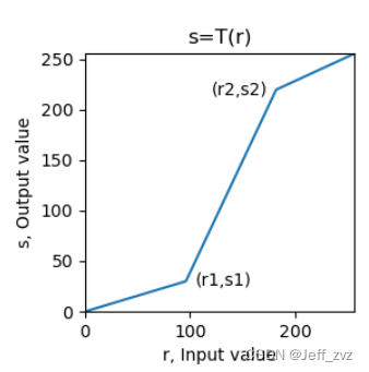

def fenduan(img,x1,x2,y1,y2):
    if x1==x2 or x2==255:
        return None
    # Mask 
    m1 = (img<x1)
    m2 = (img>=x1)& (img <= x2)
    m3 = (img>x2)

    out = (img*y1/x1)*m1 + (((img-x1)*(y2-y1)/(x2-x1))+y1)*m2 \
        +(((255-y2)*(img-x2)/(255-x2))+y2)*m3

    return out

You can also use gray levels for layering

imgLayer1[(imgLayer1[:,:]<a) | (imgLayer1[:,:]>b)] = 0  #  Other areas ： black 
imgLayer1[(imgLayer1[:,:]>=a) & (imgLayer1[:,:]<=b)] = 255  #  Grayscale window ： white 

Threshold transformation

$$\mathrm{Z}=\{\begin{array}{l}z1,x\le th1\\ z2,x>th2\end{array}\text{\hspace{1em}(1)}$$
Below a threshold , become z1; Above a certain threshold , become z2.
cv2.threshold(src,thresh,maxval,type[,dst])->retval, dst

• scr： The input image of the transform operation ,nparray Two dimensional array , Must be a single channel grayscale image ！
• thresh： threshold , Value range 0~255
• maxval： Fill color , Value range 0～255, Usually take 255
• type： Transformation type
  cv2.THRESH_BINARY： Set when greater than the threshold 255, Otherwise, set 0
  cv2.THRESH_BINARY_INV： Set when greater than the threshold 0, Otherwise, set 255
  cv2.THRESH_TRUNC： When it is greater than the threshold value, it is set as the threshold value thresh, Otherwise unchanged （ Keep the primary color ）
  cv2.THRESH_TOZERO： It does not change when it is greater than the threshold （ Keep the primary color ）, Otherwise, set 0
  cv2.THRESH_TOZERO_INV： Set when greater than the threshold 0, Otherwise unchanged （ Keep the primary color ）
  cv2.THRESH_OTSU： Use OTSU Algorithm selection threshold
• Return value retval： Returns the threshold of binarization
• Return value dst： Returns the output image of the threshold transformation

Histogram Processing

Histogram

A histogram is a graph showing the number of grayscale levels .
Normalized histogram normalizes it , Show its probability distribution .

def hist(img_c):
    r,c = img_c.shape
    img_c = img_c.flatten() # Flattening 
    img_c = img_c.tolist()
    myhist = [img_c.count(i)/(r*c) for i in range(256)] # normalization 
    return myhist

opencv Middle function
cv2.calcHist(images, channels, mask, histSize, ranges[, hist[, accumulate ]]) → hist

images： The input image , use [] Brackets indicate
channels： Histogram calculation channel , use [] Brackets indicate , The grayscale is 0
mask： mask image , It's usually set to None
histSize： Number of square columns , Usually take 256
ranges： Value range of pixel value , It's usually [0,256]
Return value hist： Returns the total number of pixels in the image for each pixel value , Shape is (histSize,1)

Histogram equalization

Histogram equalization is to change the irregular gray distribution into a regular and balanced gray distribution . The basic idea of histogram equalization is to widen the gray level which accounts for a large proportion in the image , The gray level with small proportion is compressed , Make the histogram distribution of the image more uniform , Expand the dynamic range of gray value difference , So as to enhance the overall contrast of the image .

There are conclusions in probability theory ：

When there is Z = T (\r) when , There is a probability distribution ：
$$P_z(z)=P_r(r)\ast |dz|/|dr|$$
And easy to prove
$$T(r)=(L-1)\ast {\int }_0^r{P}_w(w)dw$$
Discrete form

From the above T(\r), And the image is discrete , Transform function T(\r) Is the accumulation of probability distributions , A curve is similar to a trapezoid monotonically increasing .

def get_pdf(img): # Probability density distribution 
    total = img.shape[0]*img.shape[1]
    return [np.sum(img==i)/total for i in range(256)]

def hist_equal(img):
    pdf = get_pdf(img)
    out = np.copy(img)
    s = 0.
    Tr = [] #  Transform function 
    for i in range(256):
        s = s+pdf[i] 
        out[(img==i)] = s*255.
        Tr.append(s*255.)
    out = out.astype(np.uint8)
    return out,Tr

opencv function
cv2.equalizeHist(src[, dst]) → dst

Histogram matching ( Histogram normalization )

Suppose the graph 2 The histogram effect is the histogram we want , Our original picture is 1. It is known that we can histogram equalize the graph 1、 chart 2 All become over histogram , From the transformation function we can get the graph 2 Mapping table to transition histogram , So we can inverse map back to graph 2.

def get_pdf(img): # Probability density distribution 
    total = img.shape[0]*img.shape[1]
    return [np.sum(img==i)/total for i in range(256)]

def hist_equal(img):
    pdf = get_pdf(img)
    out = np.copy(img)
    s = 0.
    Tr = [] #  Transform function 
    for i in range(256):
        s = s+pdf[i]
        out[(img==i)] = s*255.
        Tr.append(s*255.)
    out = out.astype(np.uint8)
    return out,Tr


def gen_eq_pdf(): # Generate uniform distribution , The histogram we want 
    return [0.0039 for i in range(256)] # 1/256 = 0.0039 

def gen_target_table(Pv): #Pv To build a good probability distribution histogram 
    table = []
    # The following code is to execute G Transformation , equalization ( The vertical axis ） Map to ideal histogram （ The horizontal axis ）
    SUMq = 0.
    for i in range(256): # Known grayscale values are from 0 To 255, By transforming functions , Map to vertical axis , Form mapping table 
        SUMq = SUMq + Pv[i]
        table.append(np.round(SUMq*255,0)) # rounding 
    return table

def hist_specify(img):
    Pv = gen_eq_pdf()
    table = gen_target_table(Pv)

    ori_img,T_trans = hist_equal(img) #ori_img Namely B'

    out = ori_img.copy() # Construct output image 
    map_val = 0 # The inverse mapping value is initialized to 0
    for v in range(256):
        if v in ori_img:
            if v in table:
                map_val = len(table)-table[::-1].index(v)-1 # find , Take the largest one 
            out[(ori_img == v)] = map_val # No inverse mapping relationship found , Take the previous one 

    return out

Local histogram equalization

Histogram equalization and histogram matching are based on the global transformation of the gray distribution of the whole image , It is not for the details of the local area of the image .

Histogram processing is also applicable to local , The idea of local histogram processing is to transform the histogram based on the gray distribution of the pixel neighborhood .

The process ：

（1） Set a template of a certain size （ Rectangular neighborhood ）, Move pixel by pixel in the image ;

（2） For each pixel position , Calculate the histogram of the template area , Histogram equalization or histogram matching transformation is performed on the local region , The transformation result is only used for the gray value correction of the central pixel of the template area ;

（3） Templates （ Neighborhood ） Move line by line and column by column in the image , Traverse all pixels , Complete the local histogram processing of the whole image .

opencv function :
cv2.createCLAHE([, clipLimit[, tileGridSize]]) → retval

• clipLimit： Threshold of color contrast , optional , The default value is 8
• titleGridSize： Template for local histogram equalization （ Neighborhood ） size , optional , The default value is (8,8)

cv2. createCLAHE It is an adaptive histogram equalization method with limited contrast （Contrast Limited Adaptive Hitogram Equalization）, The method of limiting histogram distribution and accelerated interpolation are adopted .

import cv2
import numpy as np
import matplotlib.pyplot as plt

img = cv2.imread('img/low_pix.jpg',0)
imgequ = cv2.equalizeHist(img)
clahe = cv2.createCLAHE(clipLimit=2.0,tileGridSize=(4,4))
imglocalequ = clahe.apply(img)

plt.figure(figsize=(9, 6))
plt.subplot(131), plt.title('Original'), plt.axis('off')
plt.imshow(img, cmap='gray', vmin=0, vmax=255)
plt.subplot(132), plt.title(f'Global Equalize Hist'), plt.axis('off')
plt.imshow(imgequ, cmap='gray', vmin=0, vmax=255)
plt.subplot(133), plt.title(f'Local Equalize Hist'), plt.axis('off')
plt.imshow(imglocalequ, cmap='gray', vmin=0, vmax=255)
plt.tight_layout()
plt.show()

Spatial filtering

Image filtering is to suppress the noise of the target image while preserving the detailed features of the image as much as possible , It is a common image preprocessing operation .

Image smoothing and filtering

Smooth filtering is also called low-pass filtering , It can suppress the gray mutation in the image , Blur the image , It's low-frequency enhanced spatial filtering technology

Mean filtering

Mean filtering is to replace the middle value with the average value of the pixel values in the neighborhood , The side effect is to blur the image （ Blur the edges ）, And the larger the convolution kernel is, the more fuzzy it becomes .
Mathematically speaking , Because the mean filter will be affected by neighborhood points , The edge is an abrupt point of change , Therefore, the pixel values in this region become smooth after the mean filter convolution , The image is blurred .

The following is the mean filter after noise processing , Threshold processing .

Code ：
dst=cv2.blur(src ,ksize, anchor, borderType)

median filtering

Median filtering is a nonlinear smoothing technique , It is a filter based on statistical sorting method , It sorts the pixel values within the mask by one dimension , Then take the middle value as the current pixel value . Compared with the mean filter, its biggest feature is , This is an edge preserving filter , The replaced value is the original value of the image . And it can eliminate outliers , It has the best effect on salt and pepper noise .

Code ：
dst=cv2.medianBlur（src,ksize）

Bilateral filtering

Bilateral filtering is a compromise method that combines spatial proximity and pixel value similarity , At the same time, spatial information and gray similarity are considered , Denoising while effectively preserving the edges , It has a beautifying effect on portraits .

The edge gray changes greatly , Gaussian filtering will obviously blur the edge , Weak protection for high-frequency information . Bilateral filtering adds Gaussian variance of pixel intensity difference on the basis of Gaussian filtering , Pixels far away from the edge have little effect on the pixel value on the edge , To achieve edge protection .

Bilateral filtering can not filter high-frequency noise in color images well .

The mathematical formula is as follows ：

opencv function ：
cv2.bilateralFilter(src, d, sigmaColor, sigmaSpace[, dst[, borderType]]) → dst

Parameter description ：

• src： The input image , It can be a grayscale image , It can also be a multi-channel color image
• dst： Output image , Size and type versus src identical
• d： The pixel neighborhood diameter of the filter kernel . Such as d<=0 , From sigmaSpace To calculate the .
• sigmaColor： Variance of filter kernel in color space , Reflect the size of the color intensity interval that produces color influence
• sigmaSpace： Variance of filter kernel in coordinate space , Reflect the size of the influence space that produces color influence
• borderType： Type of boundary extension

Guided filtering

Guided filtering is also called guided filtering , Reflect the edge through a guide picture 、 Objects and other information , Filter the input image , The content of the output image is determined by the input image , But the texture is similar to the guide picture .

The principle of guided filtering is local linear model , While maintaining the advantages of bilateral filtering （ Effectively keep edges , Non iterative computation ） At the same time, the calculation speed is very fast , So as to overcome the disadvantage of slow bilateral filtering speed .

opencv function ：
cv2.ximgproc_guidedFilter.filter(guide, src, d[, eps[, dDepth]) → dst

Parameter description :

• src： The input image , It can be a grayscale image , It can also be a multi-channel color image
• guide： Guide image , Size and type versus src identical
• dst： Output image , Size and type versus src identical
• d： The pixel neighborhood diameter of the filter kernel
• eps： Normalized parameters , eps The square of is similar to that in bilateral filtering sigmaColor
• dDepth： The data depth of the output picture

Image sharpening and filtering

The image is blurred by smoothing （ weighted mean ） To achieve , Similar to integral operation . Image sharpening is performed by differential operation （ Finite difference ） Realization , The change value of image gray can be obtained by first-order differentiation or second-order differentiation .

The purpose of image sharpening is to enhance the gray jump part of the image , Make the blurred image clear . Image sharpening is also called high pass filtering , Through and enhancement of high frequency , Attenuate and suppress low frequencies . Image sharpening is often used in electronic printing 、 Medical imaging and industrial testing .

• Constant gray area , The first derivative is zero , The second derivative is zero ;
• Grayscale step or ramp start area , The first derivative is nonzero ,, The second derivative is nonzero ;
• Grayscale ramp area , The first derivative is nonzero , The second derivative is zero .

Mask and derivation ：

Image ,x and y Derivation of direction （ gradient ） It can be expressed by difference （ Because the image is discrete ）, Both $$\frac{\partial f}{\partial x}=f(x+1,y)-f(x,y)$$
The mask is

The second derivative is
$$\frac{{\partial }^{2}f}{\partial x^2}=f(x-1,y)+f(x+1,y)-2f(x,y)$$
Mask as

Laplace operator

$$\Delta f=\frac{{\partial }^{2}f}{\partial y^2}+\frac{{\partial }^{2}f}{\partial x^2}=f(x-1,y)+f(x+1,y)+f(x,y-1)+f(x,y+1)-4f(x,y)$$
Mask as ：

Laplace operator is a second derivative operator , The position of the edge is determined by using the quadratic differential characteristic and the zero crossing point between the peaks , More sensitive to singular points or edge points .

dst = cv2.Laplacian(src, ddepth[, dst[, ksize[, scale[, delta[, borderType]]]]])

def Laplace(img):
    edge = cv2.Laplacian(img,-1,ksize=3)
    edge = cv2.convertScaleAbs(edge)
    e_edge = cv2.equalizeHist(edge)
    out = img + e_edge
    plt.subplot(221)
    plt.imshow(img,cmap='gray')
    plt.title('original')
    plt.subplot(222)
    plt.imshow(edge,cmap='gray')
    plt.title('edge')
    plt.subplot(223)
    plt.imshow(e_edge,cmap='gray')
    plt.title('Edge enhanced')
    plt.subplot(224)
    plt.imshow(out,cmap='gray')
    plt.title('ruihua')
    plt.show()

Passivation masking

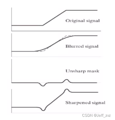
def func(img):
    blur = cv2.blur(img,(5,5))
    unsharp = img - blur 
    out = img + unsharp
    plt.subplot(221)
    plt.imshow(img,cmap='gray')
    plt.title('original')
    plt.subplot(222)
    plt.imshow(blur,cmap='gray')
    plt.title('blur')
    plt.subplot(223)
    plt.imshow(unsharp,cmap='gray')
    plt.title('unsharp')
    plt.subplot(224)
    plt.imshow(out,cmap='gray')
    plt.title('fanruihua')
    plt.show()

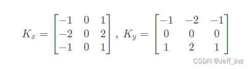
sobel operator

Sobel Operator is a discrete differential operator , It is a joint operation of Gaussian smoothing and differential derivation , Strong anti noise ability .

Sobel Gradient operator uses local difference to find edge , Calculate the approximate value of the gradient . First calculate the level 、 Vertical gradient , Then find the total gradient . Programming implementation , The square root can be approximated by the absolute value ：G = ∣ G x ∣ + ∣ G y ∣

opencv function ：
cv2.Sobel(src, ddepth, dx, dy[, dst[, ksize[, scale[, delta[, borderType]]]]]) → dst

Parameter description :

• src： The input image , Grayscale image , Not applicable to color images
• dst： Output image , Size and type versus src identical
• ddepth： The data depth of the output picture , Select by the depth of the input image
• dx：x The order of the axial derivative ,1 or 2
• dy：y The order of the axial derivative ,1 or 2
• ksize：Sobel The size of the convolution kernel , The optional values are ：1/3/5/7,ksize=-1 When using Scharr Operator operation
• scale： Scale factor , optional , The default value is 1
• delta： The offset of the output image , optional , The default value is 0
• borderType： Type of boundary extension , Note that contralateral padding is not supported （BORDER_WRAP）

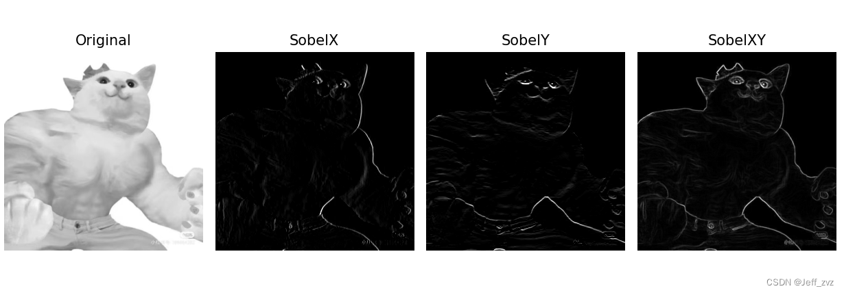
def sobel(img):
    SobelX = cv2.Sobel(img, cv2.CV_16S, 1, 0)  #  Calculation  x  Axis direction 
    SobelY = cv2.Sobel(img, cv2.CV_16S, 0, 1)  #  Calculation  y  Axis direction 
    absX = cv2.convertScaleAbs(SobelX)  #  Turn it back  uint8
    absY = cv2.convertScaleAbs(SobelY)  #  Turn it back  uint8
    SobelXY = cv2.addWeighted(absX, 0.5, absY, 0.5, 0)  #  Approximate the square root with the absolute value 
    plt.figure(figsize=(10, 6))
    plt.subplot(141), plt.axis('off'), plt.title("Original")
    plt.imshow(img, cmap='gray', vmin=0, vmax=255)

    plt.subplot(142), plt.axis('off'), plt.title("SobelX")
    plt.imshow(SobelX, cmap='gray', vmin=0, vmax=255)

    plt.subplot(143), plt.axis('off'), plt.title("SobelY")
    plt.imshow(SobelY, cmap='gray', vmin=0, vmax=255)

    plt.subplot(144), plt.axis('off'), plt.title("SobelXY")
    plt.imshow(SobelXY, cmap='gray')
    plt.tight_layout()
    plt.show()