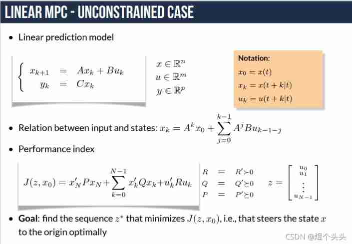
当前位置:网站首页>MPC learning notes (I): push MPC formula manually
MPC learning notes (I): push MPC formula manually
2022-06-26 08:33:00 【Yu Getou】
1. Introduce
MPC(Model Predictive Control), Model predictive control , It is an advanced process control method . Compared with LQR and PID The algorithm can only consider various constraints of input and output variables ,MPC The algorithm can consider the constraints of state space variables . It can be applied to linear and nonlinear systems .
Reference material :
2.MPC Four elements
(1) Model : Adopt step response
(2) forecast
(3) Rolling optimization :
Second planning
J ( x ) = x 2 + b x + c J\left(x\right)=x^2+bx+c J(x)=x2+bx+c
Extreme points
J ′ ( x 0 ) = 0 J^\prime\left(x_0\right)=0 J′(x0)=0
(4) Error compensation
Parameters are defined
P: Prediction step
y ( k + 1 ) , y ( k + 2 ) … y ( k + P ) y\left(k+1\right),y\left(k+2\right)\ldots y(k+P) y(k+1),y(k+2)…y(k+P)
M: Control step size
∆ u ( k ) , ∆ u ( k + 1 ) … ∆ u ( k + M ) \ ∆u(k),∆u(k+1)…∆u(k+M) ∆u(k),∆u(k+1)…∆u(k+M)
3. Derivation process
(1) Model
Assume that T,2T…PT The output corresponding to the time model is
a 1 , a 2 … a p a_1,a_2\ldots a_p a1,a2…ap
According to the superposition principle of linear system :
y ( k ) = a 1 ∗ u ( k − 1 ) + a 2 ∗ u ( k − 2 ) + a M ∗ u ( k − M ) y\left(k\right)=a_1\ast u\left(k-1\right)+a_2\ast u\left(k-2\right)+a_M\ast u(k-M) y(k)=a1∗u(k−1)+a2∗u(k−2)+aM∗u(k−M)
Incremental :
∆ y ( k ) = a 1 ∗ ∆ u ( k − 1 ) + a 2 ∗ ∆ u ( k − 2 ) + a M ∗ ∆ u ( k − M ) ∆y\left(k\right)=a_1\ast ∆u\left(k-1\right)+a_2\ast ∆u\left(k-2\right)+a_M\ast ∆u(k-M) ∆y(k)=a1∗∆u(k−1)+a2∗∆u(k−2)+aM∗∆u(k−M)
(2) forecast : A total of P A moment
∆ y ( k + 1 ) = a 1 ∗ ∆ u ( k ) ∆y(k+1)=a_1\ast∆u(k) ∆y(k+1)=a1∗∆u(k)
∆ y ( k + 2 ) = a 1 ∗ ∆ u ( k ) + 1 + a 2 ∗ ∆ u ( k ) ∆y(k+2)=a_1*∆u(k)+1+a_2*∆u(k) ∆y(k+2)=a1∗∆u(k)+1+a2∗∆u(k)
∆ y ( k + P ) = a 1 ∗ ∆ u ( k + P − 1 ) + a 2 ∗ ∆ u ( k + P − 2 ) … + a M ∗ ∆ u ( k + P − M ) ∆y(k+P)=a_1*∆u(k+P-1)+a_2*∆u(k+P-2)…+a_M*∆u(k+P-M) ∆y(k+P)=a1∗∆u(k+P−1)+a2∗∆u(k+P−2)…+aM∗∆u(k+P−M)
Turn to matrix representation :
∑ i = 1 M a i ∗ ∆ u ( k + P − i ) \sum_{i=1}^{M}{a_i\ast}∆u(k+P-i) i=1∑Mai∗∆u(k+P−i)
New forecast output = Original forecast output + Incremental input
Y ^ 0 = A ∗ ∆ u + Y 0 [ Y ^ 0 ( k + 1 ) Y ^ 0 ( k + 2 ) ⋮ Y ^ 0 ( k + P ) ] = [ a 1 0 a 2 a 1 ⋯ 0 ⋯ 0 ⋮ ⋮ a P a P − 1 ⋱ ⋮ ⋯ a P − M + 1 ] [ ∆ u ( k ) ∆ u ( k + 1 ) ⋮ ∆ u ( k + M ) ] + [ Y 0 ( k + 1 ) Y 0 ( k + 2 ) ⋮ Y 0 ( k + P ) ] {\hat{Y}}_0=A\ast∆u+Y_0 \\ \left[\begin{matrix}\begin{matrix}{\hat{Y}}_0(k+1)\\{\hat{Y}}_0(k+2)\\\end{matrix}\\\begin{matrix}\vdots\\{\hat{Y}}_0(k+P)\\\end{matrix}\\\end{matrix}\right]=\left[\begin{matrix}\begin{matrix}a_1&0\\a_2&a_1\\\end{matrix}&\begin{matrix}\cdots&0\\\cdots&0\\\end{matrix}\\\begin{matrix}\vdots&\vdots\\a_P&a_{P-1}\\\end{matrix}&\begin{matrix}\ddots&\vdots\\\cdots&a_{P-M+1}\\\end{matrix}\\\end{matrix}\right] \left[\begin{matrix}\begin{matrix}∆u(k)\\∆u(k+1)\\\end{matrix}\\\begin{matrix}\vdots\\∆u(k+M)\\\end{matrix}\\\end{matrix}\right]+\left[\begin{matrix}\begin{matrix}Y_0(k+1)\\Y_0(k+2)\\\end{matrix}\\\begin{matrix}\vdots\\Y_0(k+P)\\\end{matrix}\\\end{matrix}\right] Y^0=A∗∆u+Y0⎣⎢⎢⎢⎡Y^0(k+1)Y^0(k+2)⋮Y^0(k+P)⎦⎥⎥⎥⎤=⎣⎢⎢⎢⎡a1a20a1⋮aP⋮aP−1⋯⋯00⋱⋯⋮aP−M+1⎦⎥⎥⎥⎤⎣⎢⎢⎢⎡∆u(k)∆u(k+1)⋮∆u(k+M)⎦⎥⎥⎥⎤+⎣⎢⎢⎢⎡Y0(k+1)Y0(k+2)⋮Y0(k+P)⎦⎥⎥⎥⎤
(3) Rolling optimization
notes : Solved ∆u by M*1 Vector , Take the first one , namely ∆ u 0 ∆u_0 ∆u0 Increment as input .
Reference trajectory
Use first-order filtering :
ω ( k + i ) = α i y ( k ) + ( 1 − α i ) y r ( k ) \omega\left(k+i\right)=\alpha^iy\left(k\right)+(1-\alpha^i)y_r(k) ω(k+i)=αiy(k)+(1−αi)yr(k)Cost function ( Similar to optimal control )
Form 1Goal one : The closer you get to your goal, the better
J 1 = ∑ i = 1 P [ y ( k + i ) − ω ( k + i ) ] 2 J_1=\sum_{i=1}^{P}\left[y\left(k+i\right)-\omega\left(k+i\right)\right]^2 J1=i=1∑P[y(k+i)−ω(k+i)]2Goal two : The smaller the energy consumption, the better
J 2 = i = ∑ i = 1 M [ ∆ u ( k + i − 1 ) ] 2 J_2=i=\sum_{i=1}^{M}[∆u(k+i-1)]^2 J2=i=i=1∑M[∆u(k+i−1)]2The total cost function is obtained by combining
J = q J 1 + r J 2 J=qJ_1+rJ_2 J=qJ1+rJ2q and r Are weight coefficients , Their relative size indicates which indicator is more important , The bigger it is, the more important it is .
Matrix form :
J = ( r − ω ) T Q ( R − ω ) + ∆ u T R ∆ u J=\left(r-\omega\right)^TQ\left(R-\omega\right)+∆u^TR∆u\\ J=(r−ω)TQ(R−ω)+∆uTR∆u
among ,Q and R Most of them are diagonal matrices ( Generally, covariance matrix is not considered , That is, the interaction between different variables )
[ q 1 0 . . . 0 0 q 2 . . . 0 ⋮ ⋮ ⋱ ⋮ 0 0 0 q n ] [ r 1 0 . . . 0 0 r 2 . . . 0 ⋮ ⋮ ⋱ ⋮ 0 0 0 r n ] \begin{bmatrix} q_1& 0 & ... & 0\\ 0& q_2 & ...& 0\\ \vdots & \vdots &\ddots &\vdots \\ 0&0 & 0&q_n \end{bmatrix} \begin{bmatrix} r_1& 0 & ... & 0\\ 0& r_2 & ...& 0\\ \vdots & \vdots &\ddots &\vdots \\ 0&0 & 0&r_n \end{bmatrix} ⎣⎢⎢⎢⎡q10⋮00q2⋮0......⋱000⋮qn⎦⎥⎥⎥⎤⎣⎢⎢⎢⎡r10⋮00r2⋮0......⋱000⋮rn⎦⎥⎥⎥⎤
Optimal solution :
∂ J ( Δ u ) ∂ ( Δ u ) = 0 → Δ u = ( A T Q A + R ) − 1 A T ( ω − Y 0 ) \frac{\partial \mathrm{J}(\Delta u)}{\partial(\Delta u)}=0 \rightarrow \Delta u=\left(\mathrm{A}^{\mathrm{T}} \mathrm{QA}+\mathrm{R}\right)^{-1} \mathrm{~A}^{\mathrm{T}}\left(\omega-\mathrm{Y}_{0}\right) ∂(Δu)∂J(Δu)=0→Δu=(ATQA+R)−1 AT(ω−Y0)
Form 2- be based on u k , u k + 1 . . . u k + N − 1 Into the That's ok most optimal turn u_k,u_{k+1}...u_{k+N-1} Optimize uk,uk+1...uk+N−1 Into the That's ok most optimal turn
J = ∑ k N − 1 ( E k T Q E k + u k T R u k ) + E N T F E N ⏟ t e r m i n a l p r e d i c t s t a t u s J = \sum_k^{N-1}(E_k^TQE_k + u_k^TRu_k)+\underbrace{E_N^TFE_N} _{terminal \ predict \ status} J=k∑N−1(EkTQEk+ukTRuk)+terminal predict statusENTFEN
- be based on u k , u k + 1 . . . u k + N − 1 Into the That's ok most optimal turn u_k,u_{k+1}...u_{k+N-1} Optimize uk,uk+1...uk+N−1 Into the That's ok most optimal turn
(4) Correction feedback , Error compensation
k moment , forecast P Outputs :
Y ^ 0 ( k + 1 ) , Y ^ 0 ( k + 2 ) . . . Y ^ 0 ( k + P ) {\hat{Y}}_0\left(k+1\right),{\hat{Y}}_0\left(k+2\right)...{\hat{Y}}_0\left(k+P\right) Y^0(k+1),Y^0(k+2)...Y^0(k+P)k+1 moment , The current output is :
y ( k + 1 ) y(k+1) y(k+1)error :
e ( k + 1 ) = y ( k + 1 ) − Y ^ 0 ( k + 1 ) e\left(k+1\right)=\ y\left(k+1\right)-{\hat{Y}}_0\left(k+1\right) e(k+1)= y(k+1)−Y^0(k+1)
h: Compensation coefficient , Value range 0-1, habit 0.5
compensate :
y c o r ( k + 1 ) = Y ^ 0 ( k + 1 ) + h 1 ∗ e ( k + 1 ) y c o r ( k + 2 ) = Y ^ 0 ( k + 2 ) + h 2 ∗ e ( k + 1 ) ⋮ y c o r ( k + P ) = Y ^ 0 ( k + P ) + h P ∗ e ( k + 1 ) {y}_{cor}\left(k+1\right)=\ {\hat{Y}}_0\left(k+1\right)+h_1\ast e\left(k+1\right) \\y_{cor}\left(k+2\right)=\ {\hat{Y}}_0\left(k+2\right)+h_2\ast e\left(k+1\right) \\\vdots \\y_{cor}\left(k+P\right)=\ {\hat{Y}}_0\left(k+P\right)+h_P\ast e\left(k+1\right) ycor(k+1)= Y^0(k+1)+h1∗e(k+1)ycor(k+2)= Y^0(k+2)+h2∗e(k+1)⋮ycor(k+P)= Y^0(k+P)+hP∗e(k+1)
The matrix represents :
Y c o r = Y ^ 0 + H ∗ e ( k + 1 ) Y_{cor}={\hat{Y}}_0+H\ast e(k+1) Ycor=Y^0+H∗e(k+1)
Rolling update forecast output :
K+1 moment :
Y ^ 0 = S ∗ Y c o r {\hat{Y}}_0=S\ast Y_{cor} Y^0=S∗Ycor
S: Shift matrix (PxP)
[ 0 1 0 0 ⋯ 0 ⋯ ⋮ ⋮ ⋮ 0 0 ⋱ 1 ⋯ 1 ] \left[\begin{matrix}\begin{matrix}0&1\\0&0\\\end{matrix}&\begin{matrix}\cdots&0\\\cdots&\vdots\\\end{matrix}\\\begin{matrix}\vdots&\vdots\\0&0\\\end{matrix}&\begin{matrix}\ddots&1\\\cdots&1\\\end{matrix}\\\end{matrix}\right] ⎣⎢⎢⎢⎢⎡0010⋮0⋮0⋯⋯0⋮⋱⋯11⎦⎥⎥⎥⎥⎤
Add : Derivation of cost function

边栏推荐
- Remote centralized control of distributed sensor signals using wireless technology
- Microcontroller from entry to advanced
- Design based on STM32 works: multi-functional atmosphere lamp, wireless control ws2812 of mobile app, MCU wireless upgrade program
- Cause analysis of serial communication overshoot and method of termination
- StarWar armor combined with scanning target location
- Teach you a few tricks: 30 "overbearing" warm words to coax girls, don't look regret!
- MySQL insert Chinese error
- 1GHz active probe DIY
- [postgraduate entrance examination: planning group] clarify the relationship among memory, main memory, CPU, etc
- Interpretation of x-vlm multimodal model
猜你喜欢

51 single chip microcomputer project design: schematic diagram of timed pet feeding system (LCD 1602, timed alarm clock, key timing) Protues, KEIL, DXP
![[unity mirror] use of networkteam](/img/b8/93f55d11ea4ce2c86df01a9b03b7e7.png)
[unity mirror] use of networkteam
![[postgraduate entrance examination] group planning exercises: memory](/img/ac/5c63568399f68910a888ac91e0400c.png)
[postgraduate entrance examination] group planning exercises: memory

(3) Dynamic digital tube

Reflection example of ads2020 simulation signal

RF filter
2020-10-20

Can the encrypted JS code and variable name be cracked and restored?

STM32 project design: an e-reader making tutorial based on stm32f4
Analysis of internal circuit of operational amplifier
随机推荐
Can the encrypted JS code and variable name be cracked and restored?
Design of reverse five times voltage amplifier circuit
Parameter understanding of quad dataloader in yolov5
你为什么会浮躁
73b2d wireless charging and receiving chip scheme
Torch model to tensorflow
Undefined symbols for architecture i386与第三方编译的静态库有关
Relevant knowledge of DRF
static const与static constexpr的类内数据成员初始化
Discrete device ~ resistance capacitance
RecyclerView Item 根据 x,y 坐标得到当前position(位置)
Whale conference provides digital upgrade scheme for the event site
Detailed explanation of self attention & transformer
RF filter
2020-10-29
drf的相关知识
Text to SQL model ----irnet
STM32 based d18s20 (one wire)
How to Use Instruments in Xcode
Swift code implements method calls