当前位置:网站首页>LFM signal denoising, time-frequency analysis, filtering
LFM signal denoising, time-frequency analysis, filtering
2022-07-02 02:14:00 【VICTORY_ three hundred and twenty-one】
Preface
LFM (Linear Frequency Modulation,LFM) The signal has a large time bandwidth product , A large pulse compression ratio can be obtained , It is a signal form widely used in radar system and sonar system .
LFM The mathematical expression of the signal is :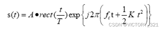
among ,A Is the signal amplitude ,t For time ,T Is the pulse duration ( Pulse width ),fc Is the carrier frequency ,K Is the linear frequency modulation rate of the signal ,rect() Rectangular window function , The mathematical expression is as follows :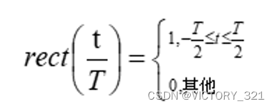
Assume signal bandwidth B=10MHz, Pulse width T=100us, Carrier frequency fc=100MHz, Sampling frequency is fs=2B=20MHz. Linear frequency modulation rate K=B/T.
The design requirements are as follows :
1. use Matlab For this parameter LFM Time frequency analysis of the signal , Come to the conclusion ;
2. Interference to signal noise ( Single frequency noise or Gaussian white noise ), Time frequency analysis of the noisy signal ;
3. Design a suitable filter , For noisy LFM The signal is filtered , Compare the effect before and after filtering .
1.LFM Time frequency analysis of signal
LFM (LFM) Signal refers to the signal whose instantaneous frequency changes linearly with time , Also known as Chirp The signal . Expression han’you With time t Item pair of t We can derive K*t, Instantaneous frequency . stay Matlab in , Generated 2000 A little long LFM The signal , Draw the real part 、 Imaginary part 、 phase 、 The instantaneous frequency is shown in the figure below :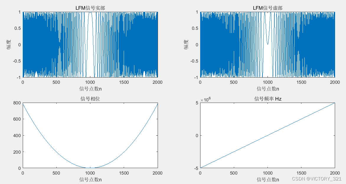
LFM The time and frequency domain waveform of the signal is as follows :
2. Add noise interference
In order to compare the influence of different kinds of noise on the signal , The addition frequency is 6MHz And Gaussian white noise ( After noise SNR=10dB).
The time domain diagram and spectrum diagram of adding single frequency noise are as follows :
Time domain diagram with Gaussian white noise 、 The spectrum diagram is as follows :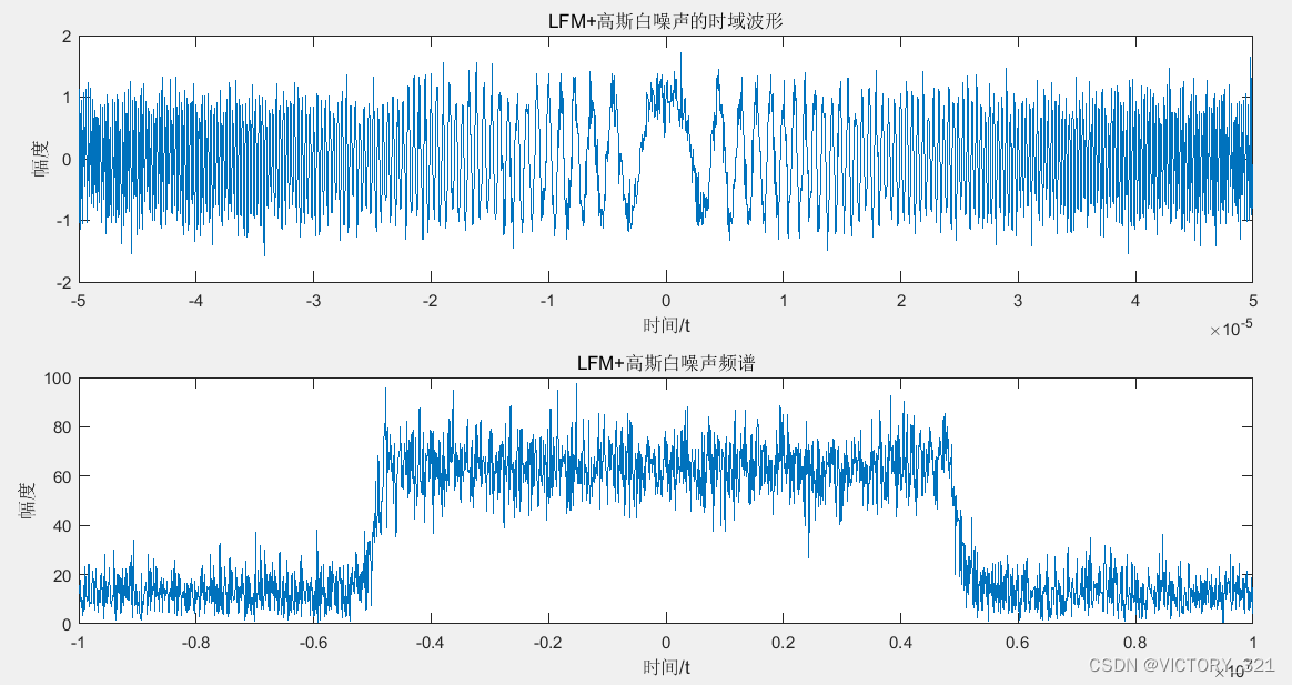
3. Noisy LFM Signal filtering
3.1 Filter out single frequency noise
utilize Matlab Inside Filter Design hold-all , To design a IIRLPF, Its low-pass frequency is 5500Hz, The cut-off frequency is 5700Hz, The stopband attenuation is 40dB.
The signal containing a single frequency is passed through the filter , Observe the output time domain diagram and frequency domain diagram .6000Hz Frequency noise is obviously filtered out , But the signal is partially distorted .
3.2 Filter the Gaussian white noise in the signal
Because the frequency of Gaussian white noise is LFM Any frequency of the signal covers , So you can't filter by filter . The commonly used method is adaptive signal filtering , for example LMS wave filtering 、RLS Filtering, etc . The principle is not repeated here . In this paper RLS Filtering method .
stay Matlab Compiling RLS The filtering procedure is as follows :
function [e,w]=my_rls(lambda,M,u,d,delta)
% recursive least squares,rls.
% Call:
% [e,w]=rls(lambda,M,u,d,delta)
%
% Input arguments:
% lambda = constant, (0,1]
% M = filter length, dim 1x1
% u = input signal, dim Nx1
% d = desired signal, dim Nx1
% delta = constant for initializaton, suggest 1e-7.
%
% Output arguments:
% e = estimation error, dim Nx1
% w = final filter coefficients, dim Mx1
% Step1:initialize
w=zeros(M,1);
P=eye(M)/delta;
u=u(:);
d=d(:);
% input signal length
N=length(u);
% error vector
e=d.';
% Step2: Loop, RLS
for n=M:N
    uvec=u(n:-1:n-M+1);
    e(n)=d(n)-w'*uvec;
    k=lambda^(-1)*P*uvec/(1+lambda^(-1)*uvec'*P*uvec);
    P=lambda^(-1)*P-lambda^(-1)*k*uvec'*P;
    w=w+k*conj(e(n));
end
Before filtering 、 After LFM The time domain diagram of the signal is as follows :
Filtered LFM The signal spectrum is as follows :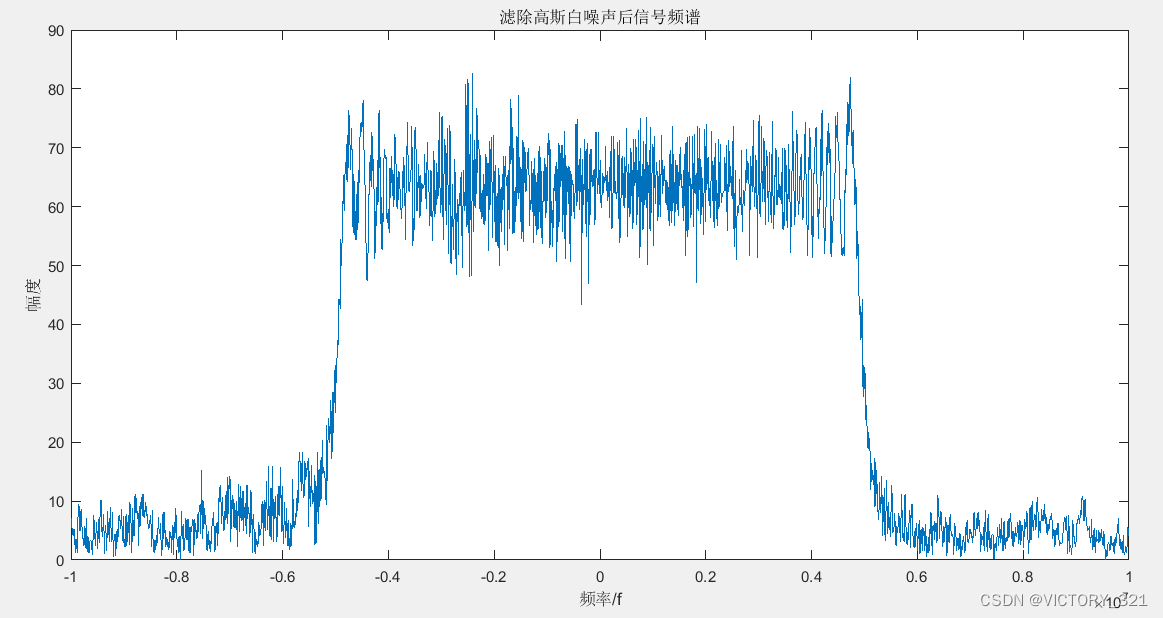
( The simulation analysis is left to everyone !)
Code
clear;
clc;
close all;
%%  Parameter setting
B=10e6;    % Signal bandwidth 10MHz
tao=10e-5;   % Pulse width 100us
fs=2*B;    % sampling frequency
Ts=1/fs;   % Sampling period
K=B/tao;     % Linear frequency modulation rate
fc =1e8;   % Carrier frequency
%%  produce LFM The signal
t=-tao/2:1/fs:tao/2-1/fs;
LFM=exp(j*2*pi*(fc*t+0.5*K*t.^2));  % Send a signal
theta =  pi*K*t.^2;      % Signal radian
ft = K*t;                 % signal frequency

figure();
subplot(2,2,1);
plot(real(LFM));
xlabel(' Signal points n');ylabel(' Range ');
title('LFM Signal real part ');
subplot(2,2,2);
plot(imag(LFM));
xlabel(' Signal points n');ylabel(' Range ');
title('LFM Imaginary part of signal ');
subplot(2,2,3);
plot(theta);
xlabel(' Signal points n');
title(' Signal phase ');
subplot(2,2,4);
plot(ft);
xlabel(' Signal points n');
title(' signal frequency  Hz');

X=fftshift(fft(LFM));
f=linspace(0,fs,length(t))-fs/2;        % Set the frequency variable
figure();
subplot(211);
plot(t,real(LFM));
xlabel(' Time /t');ylabel(' Range ');
title('LFM Signal time domain ');
subplot(212);
plot(f,abs(X));
xlabel(' frequency /f');ylabel(' Range ');
title('LFM Signal spectrum ');

%%  Add a single frequency noise
fn1=6e6;        % Noise frequency 6MHz
n1=0.1*cos(2*pi*fn1*t);
S1=LFM+n1;
figure();
subplot(211);
plot(t,S1);
xlabel(' Time /t');ylabel(' Range ');
title(' Time domain of noisy signal ');
subplot(212);
plot(f,abs(fftshift(fft(S1))));
xlabel(' frequency /f');ylabel(' Range ');
title(' Signal spectrum after noise ');

%%  Design bandpass filter
y=filter(IIRBPF2,S1);       % use Matlab Self contained filter design hold-all , Design low-pass filter , The code is shown IIRBPF2.m
[b,a]=tf(IIRBPF2);        % Put the low-pass filter IIRBPF2 Into a transfer function , The coefficient is b,a
figure();
freqz(b,a);     % do IIRBPF2  Amplitude frequency characteristic curve

figure();
subplot(211);
plot(t,y);
xlabel(' Time /t');ylabel(' Range ');
title(' Time domain diagram of denoised signal ');
subplot(212)
plot(f,abs(fftshift(fft(y))));  % Denoised spectrum
xlabel(' frequency /f');ylabel(' Range ');
title(' Denoised signal spectrum ');
%%  Add Gaussian white noise
S2=awgn(LFM,10,'measured');    % Add Gaussian white noise , The SNR is 10dB
sn=S2-LFM;                     % noise

figure();
subplot(211);
plot(t,S2);
xlabel(' Time /t');ylabel(' Range ');
title('LFM+ Time domain waveform of Gaussian white noise ');
subplot(212);
plot(f,abs(fftshift(fft(S2))));
xlabel(' Time /t');ylabel(' Range ');
title('LFM+ Gaussian white noise spectrum ');

%% RLS Algorithm filtering
mu2=0.002;
M=2;
espon=1e-5;
delta=1e-7;
lambda=0.99;
[en,w2]=my_rls(lambda,M,sn,S2,delta);%RLS Algorithm subroutine
er=en-LFM;            %er For error signal , Filter output - Input
figure();
subplot(311);
plot(t,S2);
xlabel(' Time /t');ylabel(' Range ');
title('LFM+ Time domain waveform of Gaussian white noise ');
subplot(312);
plot(t,en);
xlabel(' Time /t');ylabel(' Range ');
title(' Time domain waveform of filtered signal ');
subplot(313);
plot(t,er);
xlabel(' Time /t');ylabel(' Range ');
title(' Error signal ');

figure;
plot(f,abs(fftshift(fft(en))));
xlabel(' frequency /f');ylabel(' Range ');
title(' Signal spectrum after filtering Gaussian white noise ');
边栏推荐
- C language 3-7 daffodils (enhanced version)
- Webgpu (I): basic concepts
- How to turn off debug information in rtl8189fs
- MySQL如何解决delete大量数据后空间不释放的问题
- Construction and maintenance of business websites [15]
- how to add one row in the dataframe?
- Pytest testing framework
- How to solve MySQL master-slave delay problem
- Kibana操控ES
- The concepts and differences between MySQL stored procedures and stored functions, as well as how to create them, the role of delimiter, the viewing, modification, deletion of stored procedures and fu
猜你喜欢
![[opencv] - comprehensive examples of five image filters](/img/c7/aec9f2e03a17c22030d7813dd47c48.png)
[opencv] - comprehensive examples of five image filters
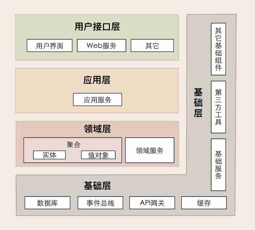
Architecture evolution from MVC to DDD

Which is a good Bluetooth headset of about 300? 2022 high cost performance Bluetooth headset inventory

【读书笔记】程序员修炼手册—实战式学习最有效(项目驱动)

附加:信息脱敏;

A quick understanding of analog electricity

RTL8189FS如何关闭Debug信息
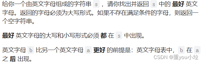
leetcode2309. 兼具大小写的最好英文字母(简单,周赛)

医药管理系统(大一下C语言课设)
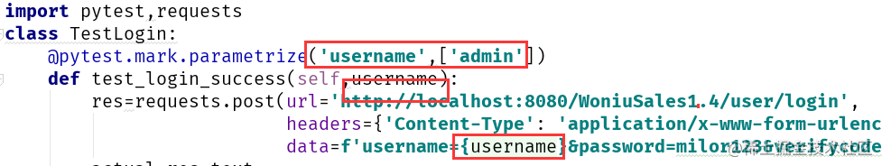
pytest 测试框架
随机推荐
MySQL中一条SQL是怎么执行的
Duplicate keys detected: ‘0‘. This may cause an update error. found in
Opengauss database backup and recovery guide
leetcode2312. Selling wood blocks (difficult, weekly race)
Decipher the AI black technology behind sports: figure skating action recognition, multi-mode video classification and wonderful clip editing
Medical management system (C language course for freshmen)
STM32F103 - two circuit PWM control motor
Redis环境搭建和使用的方法
C language 3-7 daffodils (enhanced version)
Automatically browse pinduoduo products
leetcode2309. The best English letters with both upper and lower case (simple, weekly)
MySQL constraints and multi table query example analysis
DNS domain name resolution
leetcode2309. 兼具大小写的最好英文字母(简单,周赛)
C write TXT file
AR增强现实可应用的场景
2022 Q2 - 提升技能的技巧总结
1222. Password dropping (interval DP, bracket matching)
flutter 中間一個元素,最右邊一個元素
2022 Q2 - 提昇技能的技巧總結