Machine learning notes - trend components of time series

One 、 What is the trend ？

         The trend component of the time series represents the duration of the mean value of the series 、 Long term change . The trend is the slowest part of the series , Represents the importance of the maximum time scale . In the time series of product sales , As more and more people know about this product , The impact of market expansion may be an increasing trend .

Trend patterns in four time series .

          ad locum , We will focus on the trend of the mean . More generally , Any continuous and slow-moving change in a sequence may constitute a trend —— for example , Time series usually have trends in their changes .

Two 、 Moving average chart

         To see what trends a time series might have , We can use the moving average graph . To calculate the moving average of the time series , We calculate the average of the values in a sliding window that defines the width . Each point on the chart represents the average of all values in the series located in either side of the window . The idea is to eliminate any short-term fluctuations in the sequence , So as to retain only long-term changes .

A moving average chart illustrating a linear trend . Every point on the curve （ Blue ） It's the size of 12 Point in the window of （ Red ） Average value .

          Notice the top Mauna Loa How the series repeats up and down year after year —— A short-term seasonal change . To make change part of the trend , It should take longer than any seasonal change . therefore , To visualize trends , We averaged over a longer period of time than any seasonal cycle in the series . about Mauna Loa series , We chose a size of 12 Windows to smooth the seasons of the year .

3、 ... and 、 Engineering trends

         Once we have determined the shape of the trend , We can try to use the time step feature to model it . We have seen how to use the time virtual model itself to simulate linear trends ：

target = a * time + b

         We can fit many other types of trends through the transformation of time dummy variables . If the trend seems to be quadratic （ parabola ）, We just add the square of the time dummy variable to the feature set , obtain ：

target = a * time ** 2 + b * time + c

         Linear regression will learn the coefficient a、b and c.

         The trend curves in the figure below use these features and scikit-learn Of LinearRegression Fitting ：

Top ： Series with linear trend . The figure below ： Series with secondary trend .

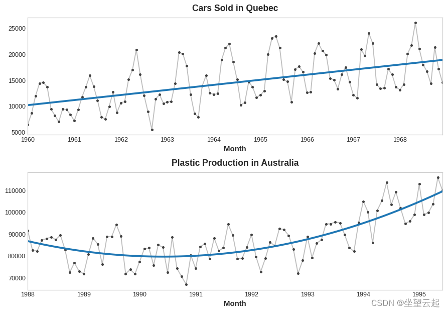
          If you haven't seen this technique before , Then you may not realize that linear regression can fit curves other than straight lines . The idea is , If you can provide a curve of appropriate shape as a feature , Then linear regression can learn how to combine them in a way that best suits the target .

Four 、 Example - Tunnel flow

         In this case , We will create a trend model for the tunnel traffic data set .

from pathlib import Path
from warnings import simplefilter

import matplotlib.pyplot as plt
import numpy as np
import pandas as pd

simplefilter("ignore")  # ignore warnings to clean up output cells

# Set Matplotlib defaults
plt.style.use("seaborn-whitegrid")
plt.rc("figure", autolayout=True, figsize=(11, 5))
plt.rc(
    "axes",
    labelweight="bold",
    labelsize="large",
    titleweight="bold",
    titlesize=14,
    titlepad=10,
)
plot_params = dict(
    color="0.75",
    style=".-",
    markeredgecolor="0.25",
    markerfacecolor="0.25",
    legend=False,
)
%config InlineBackend.figure_format = 'retina'


# Load Tunnel Traffic dataset
data_dir = Path("../input/ts-course-data")
tunnel = pd.read_csv(data_dir / "tunnel.csv", parse_dates=["Day"])
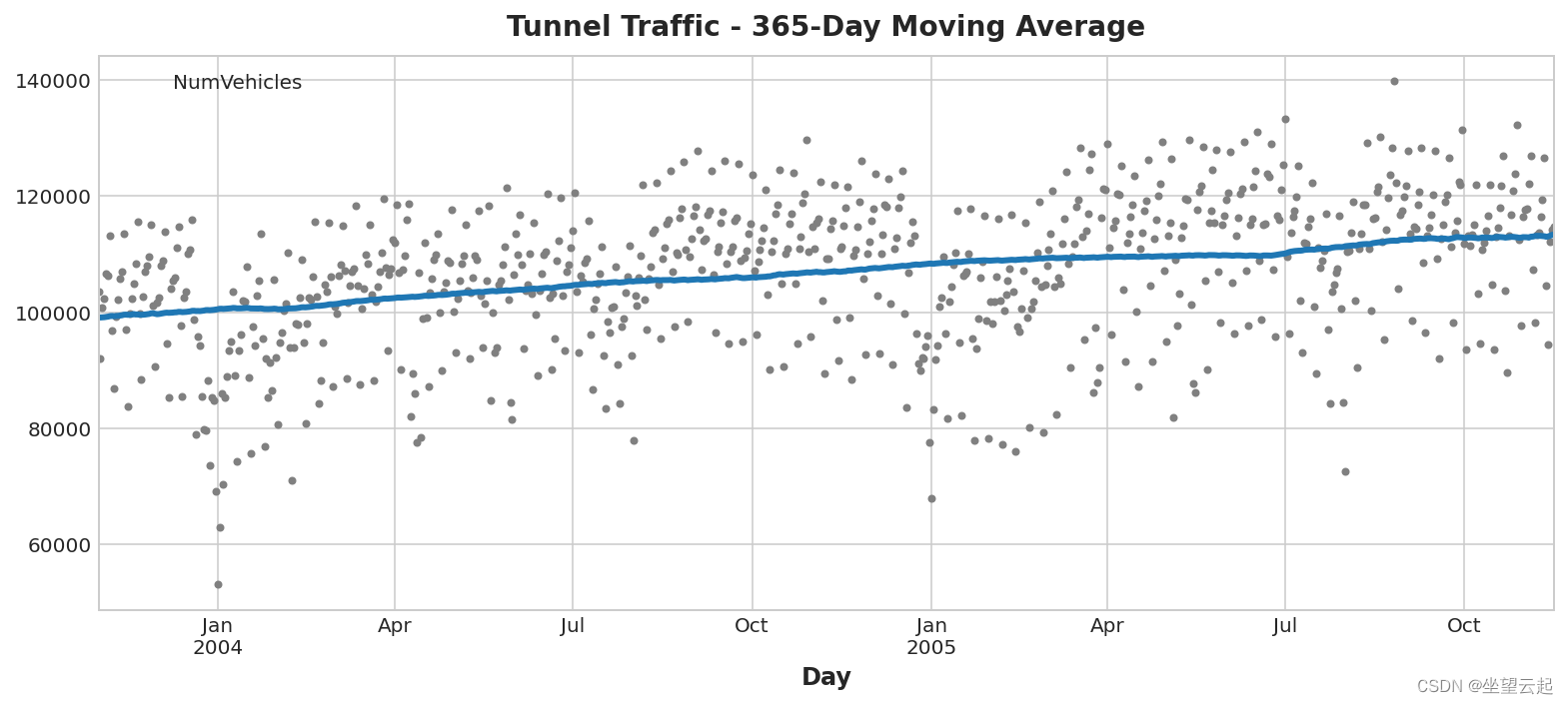
tunnel = tunnel.set_index("Day").to_period()

         Let's make a moving average , See what trends this series has . Because this series has daily observations , Let's choose one 365 A window of days to smooth out any short-term changes in a year .

         To create a moving average , First, use the scrolling method to start the window calculation . Calculate the average value of the window according to this method . As we can see , The trend of tunnel flow seems to be linear .

moving_average = tunnel.rolling(
    window=365,       # 365-day window
    center=True,      # puts the average at the center of the window
    min_periods=183,  # choose about half the window size
).mean()              # compute the mean (could also do median, std, min, max, ...)

ax = tunnel.plot(style=".", color="0.5")
moving_average.plot(
    ax=ax, linewidth=3, title="Tunnel Traffic - 365-Day Moving Average", legend=False,
);

         In the last article on time series , We are directly in the Pandas Our time virtual machine is designed in . However , from now on , We will use statsmodels One of the libraries is called DeterministicProcess Function of . Using this function will help us avoid some tricky failure cases , These cases may occur with time series and linear regression . order Parameters refer to polynomial order ：1 It means linear ,2 Indicates secondary ,3 It means three times , And so on . 

from statsmodels.tsa.deterministic import DeterministicProcess

dp = DeterministicProcess(
    index=tunnel.index,  # dates from the training data
    constant=True,       # dummy feature for the bias (y_intercept)
    order=1,             # the time dummy (trend)
    drop=True,           # drop terms if necessary to avoid collinearity
)
# `in_sample` creates features for the dates given in the `index` argument
X = dp.in_sample()

X.head()

Day	const	trend
2003-11-01	1.0	1.0
2003-11-02	1.0	2.0
2003-11-03	1.0	3.0
2003-11-04	1.0	4.0
2003-11-05	1.0	5.0

        （ By the way , A deterministic process is a technical term for a nonrandom or completely deterministic time series , It's like const Same as trend series . Characteristics derived from time indices are usually deterministic .）

         We basically create the trend model as before , But please note that fit_intercept=False Parameters .

from sklearn.linear_model import LinearRegression

y = tunnel["NumVehicles"]  # the target

# The intercept is the same as the `const` feature from
# DeterministicProcess. LinearRegression behaves badly with duplicated
# features, so we need to be sure to exclude it here.
model = LinearRegression(fit_intercept=False)
model.fit(X, y)

y_pred = pd.Series(model.predict(X), index=X.index)

         Our linear regression model found almost the same trend as the moving average graph , This shows that the linear trend is the right decision in this case .

ax = tunnel.plot(style=".", color="0.5", title="Tunnel Traffic - Linear Trend")
_ = y_pred.plot(ax=ax, linewidth=3, label="Trend")

         In order to make predictions , We apply the model to “ Out of sample ” features . “ Out of sample ” It refers to the time beyond the observation period of training data . Here's how we do it 30 Day prediction method ：

X = dp.out_of_sample(steps=30)
y_fore = pd.Series(model.predict(X), index=X.index)
y_fore.head()

2005-11-17    114981.801146
2005-11-18    115004.298595
2005-11-19    115026.796045
2005-11-20    115049.293494
2005-11-21    115071.790944
Freq: D, dtype: float64

         Let's draw part of this series to see the future 30 Day trend forecast ：

ax = tunnel["2005-05":].plot(title="Tunnel Traffic - Linear Trend Forecast", **plot_params)
ax = y_pred["2005-05":].plot(ax=ax, linewidth=3, label="Trend")
ax = y_fore.plot(ax=ax, linewidth=3, label="Trend Forecast", color="C3")
_ = ax.legend()

         Why trend models are useful , There are many reasons . In addition to serving as a baseline or starting point for more complex models , We can also use them as “ hybrid model ” One of the components in , The algorithm cannot learn the trend （ Such as XGBoost And random forest ）.