MySQL advanced optimization 01 - 40000 word detailed database performance analysis tool (in-depth, comprehensive and detailed, for collection and standby)

front said
Author's brief introduction ： Half old 518, Long distance runner , Determined to persist in writing 10 Blog of the year , Focus on java Back end
Column Introduction ：mysql Advanced , Main explanation mysql Database advanced knowledge , Include index 、 Database tuning 、 Sub warehouse, sub table, etc
The article brief introduction ： This article will introduce the steps of database optimization 、 Ideas 、 Performance analysis tool , For example, slow query 、EXPLAIN,SHOW PROFILING etc. , The performance analysis results and performance parameters of each tool are introduced and explained in detail 、 It is recommended to store it for future use .
Related to recommend ：

• MySql Advanced index 01—— Explain the data structure of the index in depth ：B+ Trees
• Mysql Advanced index 02——InnoDB The data storage structure of storage engine
• Mysql Advanced index 03——2 A new feature ,11+7 Design principles for creating indexes

1. Database server optimization steps

The whole process of database optimization is divided into Observe （Show status） and action （Action） Two parts . The database optimization can be summarized as the following figure . Letter S Part of represents observation （ Will use the corresponding analysis tools ）, Letter A The representative part is action （ Actions that can be taken by correspondence analysis ）.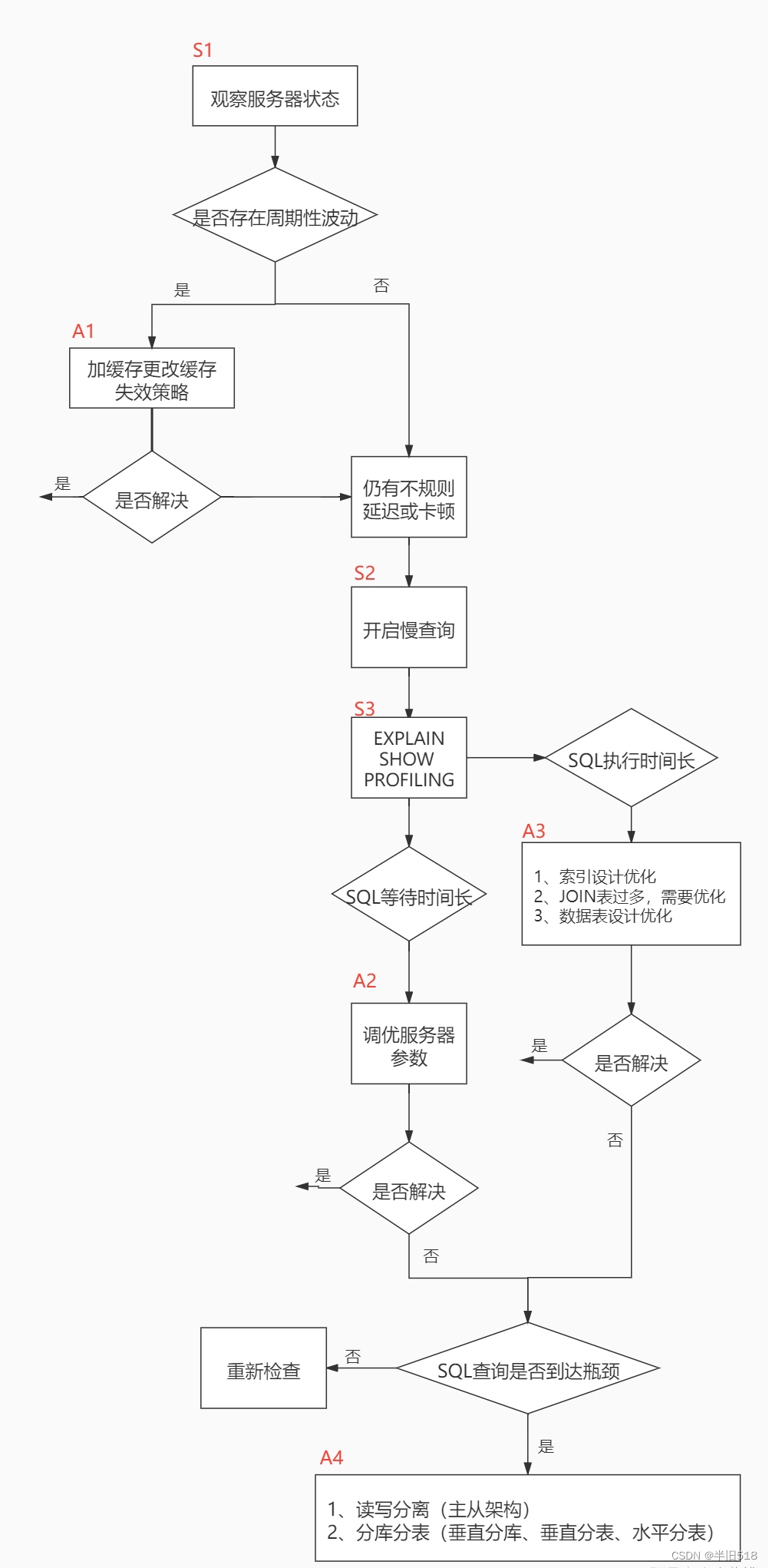

You can see from the figure , Many analysis tools are needed in the whole process : For example, slow query ,EXPLAIN,SHOW PROFILING etc. , This article will introduce these database performance analysis tools .
A brief summary is as follows ：

You can see that the steps of database tuning are moving towards the top of the pyramid , The higher the cost , The worse the effect , So we are in the process of database tuning , Focus on the bottom of the pyramid sql And index tuning , Database table structure tuning , System configuration parameter tuning And other software level tuning .

2. View system performance parameters

have access to SHOW STATUS Statement to query some database servers performance parameter and Frequency of use .
The syntax is as follows ：

SHOW [GLOBAL][SESSION] STATUES LIKE ' Parameters ';

Some common performance parameters are as follows ：

• Connections： Connect MySQL The number of servers .
• Uptime：MySQL The online time of the server .
• Slow_queries： The number of slow queries .
• Innodb_rows_read：Select The number of rows returned by the query
• Innodb_rows_inserted： perform INSERT The number of rows inserted by the operation
• Innodb_rows_updated： perform UPDATE Number of rows updated by operation
• Innodb_rows_deleted： perform DELETE The number of rows deleted by the operation
• Com_select： Number of query operations .
• Com_insert： The number of insert operations . For batch inserted INSERT operation , Only add up once .
• Com_update： The number of update operations .
• Com_delete： The number of delete operations .

Take a few examples , Play with . see mysql On line time of

mysql> show status like 'connections';
+---------------+-------+
| Variable_name | Value |
+---------------+-------+
| Connections   | 9     |
+---------------+-------+
1 row in set (0.01 sec)

Look at the number of rows added, deleted, modified and queried by the storage engine .

mysql> show status like  'innodb_rows_%';
+----------------------+-------+
| Variable_name        | Value |
+----------------------+-------+
| Innodb_rows_deleted  | 0     |
| Innodb_rows_inserted | 0     |
| Innodb_rows_read     | 8     |
| Innodb_rows_updated  | 0     |
+----------------------+-------+
4 rows in set (0.00 sec)

3. Statistics SQL The cost of searching ：last_query_cost

Let's create the data first ( A friendly reminder ： The last article has been written , If you followed the previous article , No need to rebuild .)

CREATE DATABASE atguigudb1;

USE atguigudb1;

CREATE FUNCTION rand_string(n INT)
	RETURNS VARCHAR(255) # This function returns a string 
BEGIN
	DECLARE chars_str VARCHAR(100) DEFAULT 'abcdefghijklmnopqrstuvwxyzABCDEFJHIJKLMNOPQRSTUVWXYZ';
	DECLARE return_str VARCHAR(255) DEFAULT '';
	DECLARE i INT DEFAULT 0;
	WHILE i < n DO
	   SET return_str =CONCAT(return_str,SUBSTRING(chars_str,FLOOR(1+RAND()*52),1));
	   SET i = i + 1;
    END WHILE;
    RETURN return_str;
END //


CREATE FUNCTION rand_num (from_num INT ,to_num INT) RETURNS INT(11)
BEGIN 
DECLARE i INT DEFAULT 0; 
SET i = FLOOR(from_num +RAND()*(to_num - from_num+1))  ;
RETURN i; 
END //

#  stored procedure 1： Create and insert a course schedule stored procedure 
DELIMITER //
CREATE PROCEDURE insert_course( max_num INT )
BEGIN 
	DECLARE i INT DEFAULT 0; 
	SET autocommit = 0;   # Set up manual commit transactions 
	REPEAT  # loop 
	SET i = i + 1;  # assignment 
	INSERT INTO course (course_id, course_name ) VALUES
	(rand_num(10000,10100),rand_string(6)); 
	UNTIL i = max_num 
	END REPEAT; 
	COMMIT;  # Commit transaction 
END //
DELIMITER ;

#  stored procedure 2： Create a stored procedure to insert the student table 
CREATE PROCEDURE insert_stu( max_num INT )
BEGIN 
	DECLARE i INT DEFAULT 0; 
	SET autocommit = 0;   # Set up manual commit transactions 
	REPEAT  # loop 
	SET i = i + 1;  # assignment 
	INSERT INTO student_info (course_id, class_id ,student_id ,NAME ) VALUES
(rand_num(10000,10100),rand_num(10000,10200),rand_num(1,200000),rand_string(6)); 
	UNTIL i = max_num 
	END REPEAT; 
	COMMIT;  # Commit transaction 
END //

#  Insert course data 
CALL insert_course(100);
# Insert student data 
CALL insert_stu(1000000);

Perform a query operation and view sql Execution cost ,Value Express I/O Number of data pages loaded .

mysql> select * from student_info where id = 900001;
+--------+------------+--------+-----------+----------+---------------------+
| id     | student_id | name   | course_id | class_id | create_time         |
+--------+------------+--------+-----------+----------+---------------------+
| 900001 |     128284 | jbCKPX |     10080 |    10001 | 2022-05-31 11:01:54 |
+--------+------------+--------+-----------+----------+---------------------+
1 row in set (0.00 sec)

mysql> show status like 'last_query_cost';
+-----------------+----------+
| Variable_name   | Value    |
+-----------------+----------+
| Last_query_cost | 1.000000 |
+-----------------+----------+
1 row in set (0.00 sec)

Another big one .

mysql>  select * from student_info where id between 900001 and 900100;
+--------+------------+--------+-----------+----------+---------------------+
| id     | student_id | name   | course_id | class_id | create_time         |
+--------+------------+--------+-----------+----------+---------------------+
| 900001 |     128284 | jbCKPX |     10080 |    10001 | 2022-05-31 11:01:54 |
// ...
| 900099 |      45120 | MZOSay |     10081 |    10026 | 2022-05-31 11:01:54 |
| 900100 |      83397 | lQyTXg |     10034 |    10058 | 2022-05-31 11:01:54 |
+--------+------------+--------+-----------+----------+---------------------+
100 rows in set (0.00 sec)

mysql> show status like 'last_query_cost';
+-----------------+-----------+
| Variable_name   | Value     |
+-----------------+-----------+
| Last_query_cost | 41.136003 |
+-----------------+-----------+
1 row in set (0.00 sec)

I don't know if you found out , The number of query pages above is just 41 times , However, the efficiency of query has not changed significantly , Actually these two SQL The query time is basically the same , Inquire about last_query_cost It is very useful for comparing costs , Especially when we have several query methods to choose from .

SQL Query is a dynamic process , From the point of view of page loading , We can draw the following two conclusions ：
1. Location determines efficiency : Database buffer pool > Memory > disk .
2. Batch decision efficiency ： Sequential read > Greater than random read , Sometimes reading multiple pages in batch order is even faster than loading one page randomly .
In actual production , We can take advantage of this feature , Put the data often used for query in Buffer pool in , Secondly, we can make full use of the throughput capacity of disk , Bulk read data .

4. Location execution is slow SQL： Slow query log

The slow query log is used to record statements whose corresponding time exceeds the threshold , It can help us find those that take a long time to execute sql sentence , With a view to targeted optimization . commonly mysql The slow query log of is turned off by default , It is not recommended to enable in case of non tuning , Avoid affecting the performance of the database .

4.1 Open slow query log

1️⃣ Turn on slow_query_log

see

mysql> show variables like '%slow_query_log%';
+---------------------+------------------------------------------------------+
| Variable_name       | Value                                                |
+---------------------+------------------------------------------------------+
| slow_query_log      | OFF                                                  |
| slow_query_log_file | D:\mysql-5.7.26-winx64\data\DESKTOP-1PB99O1-slow.log |
+---------------------+------------------------------------------------------+
2 rows in set, 1 warning (0.00 sec)

modify , Pay attention to the addition of global, Because it is a global system variable , Otherwise, an error will be reported .

mysql> set global slow_query_log='ON';
Query OK, 0 rows affected (0.02 sec)

Check it again .

mysql> show variables like '%slow_query_log%';
+---------------------+------------------------------------------------------+
| Variable_name       | Value                                                |
+---------------------+------------------------------------------------------+
| slow_query_log      | ON                                                   |
| slow_query_log_file | D:\mysql-5.7.26-winx64\data\DESKTOP-1PB99O1-slow.log |
+---------------------+------------------------------------------------------+
2 rows in set, 1 warning (0.00 sec)

2️⃣ modify long_query_time threshold

see .

mysql> show variables like '%long_query_time%';
+-----------------+-----------+
| Variable_name   | Value     |
+-----------------+-----------+
| long_query_time | 10.000000 |
+-----------------+-----------+
1 row in set, 1 warning (0.02 sec)

modify .

mysql> set global long_query_time = 1;
Query OK, 0 rows affected (0.00 sec)

Check it again .

mysql> show global variables like '%long_query_time%';
+-----------------+----------+
| Variable_name   | Value    |
+-----------------+----------+
| long_query_time | 1.000000 |
+-----------------+----------+
1 row in set, 1 warning (0.00 sec)

Remember to add global, Otherwise, the default is only in the current session , however , Even if you add global The above changes are only temporary , When the database server restarts , The above modification will be invalid . To be effective permanently , You need to change my.cnf file , Then restart the database server .

slow_query_log=ON
slow_query_log_file=/var/lib/mysql/atguigu-slow.log
long_query_time=3
log_output=FILE

4.2 Case presentation

1️⃣ Build table

CREATE TABLE `student` (
	`id` INT(11) NOT NULL AUTO_INCREMENT,
	`stuno` INT NOT NULL ,
	`name` VARCHAR(20) DEFAULT NULL,
	`age` INT(3) DEFAULT NULL,
	`classId` INT(11) DEFAULT NULL,
	PRIMARY KEY (`id`)
) ENGINE=INNODB AUTO_INCREMENT=1 DEFAULT CHARSET=utf8;

2️⃣ Set parameters log_bin_trust_function_creators

( The first 3 Section has been completed )

Create a function , If it's wrong

This function has none of DETERMINISTIC......

Command on ： Allows you to create function settings ：

set global log_bin_trust_function_creators=1;   #  No addition global Only the current window is valid .

3️⃣ Create a function

( The first 3 Section has been completed )
Randomly generate strings ：

DELIMITER //
CREATE FUNCTION rand_string(n INT)
RETURNS VARCHAR(255) # This function returns a string 
BEGIN
DECLARE chars_str VARCHAR(100) DEFAULT
'abcdefghijklmnopqrstuvwxyzABCDEFJHIJKLMNOPQRSTUVWXYZ';
DECLARE return_str VARCHAR(255) DEFAULT '';
DECLARE i INT DEFAULT 0;
WHILE i < n DO
   SET return_str =CONCAT(return_str,SUBSTRING(chars_str,FLOOR(1+RAND()*52),1));
   SET i = i + 1;
  END WHILE;
  RETURN return_str;
END //
DELIMITER ;
# test 
SELECT rand_string(10);

Random values are generated ( The first 3 Section has been completed )：

DELIMITER //
CREATE FUNCTION rand_num (from_num INT ,to_num INT) RETURNS INT(11)
BEGIN 
DECLARE i INT DEFAULT 0; 
SET i = FLOOR(from_num +RAND()*(to_num - from_num+1))  ;
RETURN i; 
END //
DELIMITER ;
# test ：
SELECT rand_num(10,100);

4️⃣ Create stored procedure

DELIMITER //
CREATE PROCEDURE insert_stu1(  START INT , max_num INT )
BEGIN 
DECLARE i INT DEFAULT 0; 
SET autocommit = 0;   # Set up manual commit transactions 
REPEAT  # loop 
SET i = i + 1;  # assignment 
INSERT INTO student (stuno, NAME ,age ,classId ) VALUES
((START+i),rand_string(6),rand_num(10,100),rand_num(10,1000)); 
UNTIL i = max_num 
END REPEAT; 
COMMIT;  # Commit transaction 
END //
DELIMITER ;

step 5： Calling stored procedure

# Call the function just written , 4000000 Bar record , from 100001 The start 
mysql> CALL insert_stu1(100001,4000000);
Query OK, 0 rows affected (10 min 47.03 sec)

Be careful , It will take a long time , Please be patient for a few minutes . After that, you can query whether the insertion is successful .

select count(*) from student;

There is a small detail here , The above statement for querying data volume is used in the storage engine MyISAM It is better to use InnoDB Much faster , This is because MyISAM The storage engine will have a field dedicated to the number of records .

Next, perform the following query operation , Create slow query scenarios .

mysql> set  long_query_time = 1;
Query OK, 0 rows affected (0.00 sec)

mysql> SELECT * FROM student WHERE stuno = 3455655;
+---------+---------+--------+------+---------+
| id      | stuno   | name   | age  | classId |
+---------+---------+--------+------+---------+
| 3355654 | 3455655 | QQFFkl |   57 |     904 |
+---------+---------+--------+------+---------+
1 row in set (3.47 sec)

mysql> select * from student where name = 'QQFFkl';
+---------+---------+--------+------+---------+
| id      | stuno   | name   | age  | classId |
+---------+---------+--------+------+---------+
|  143213 |  243214 | qQffkL |   95 |     543 |
|  225733 |  325734 | qQffkL |   10 |     861 |
|  280275 |  380276 | QqfFKL |   50 |     118 |
| 1355465 | 1455466 | QqfFKL |   52 |     195 |
| 1676763 | 1776764 | qQffkL |   11 |     906 |
| 1766208 | 1866209 | qqFfKl |   11 |     396 |
| 1870789 | 1970790 | qqFfKl |   97 |     182 |
| 2368740 | 2468741 | QQFFkl |   51 |     645 |
| 2386799 | 2486800 | qQffkL |   11 |     875 |
| 3170932 | 3270933 | QqfFKL |   50 |      92 |
| 3355654 | 3455655 | QQFFkl |   57 |     904 |
| 3966226 | 4066227 | qQffkL |   96 |     629 |
+---------+---------+--------+------+---------+

View the slow query records .

mysql> show status like 'slow_queries';
+---------------+-------+
| Variable_name | Value |
+---------------+-------+
| Slow_queries  | 2     |
+---------------+-------+
1 row in set (0.00 sec)

Add ： stay Mysql in , There is another variable min_examined_row_limit Used to control slow query logs , What he means is , In the query , Query time exceeds long_query_time Log , It is also necessary to ensure that the number of records scanned by the query meets min_examined_row_limit Will be recorded in the slow query log . Generally, it defaults to 0, We don't usually modify it .

SHOW VARIABLES like 'min%'
OK
 Time : 0.002s

4.3 Slow query log analysis tool ：Mysqldumpslow

In the production environment , If you want to analyze the log manually , lookup 、 analysis SQL, It's obviously individual work ,MySQL Provides log analysis tools mysqldumpslow.

Be careful :
1. The tool is not mysql Built in , Not in mysql perform , It can be executed directly in the root directory or other locations
2. The tool only has Linux The following is available for unpacking , Actually in production mysql The database is generally deployed in linux In the environment . If you are windows In the environment , You can refer to the blog https://www.cnblogs.com/-mrl/p/15770811.html.

adopt mysqldumpslow You can view the slow query log help .

mysqldumpslow --help

Maximizing growth .

Now let's use , Find the location of the slow query log first .( notes ： The author is actually windows Environment , Please refer to the blog mentioned above when using , I won't repeat it later )

mysql> show variables like '%slow_query_log%';
+---------------------+------------------------------------------------------+
| Variable_name       | Value                                                |
+---------------------+------------------------------------------------------+
| slow_query_log      | ON                                                   |
| slow_query_log_file | D:\mysql-5.7.26-winx64\data\DESKTOP-1PB99O1-slow.log |
+---------------------+------------------------------------------------------+
2 rows in set, 1 warning (0.00 sec)

Before we find it 10 Bar record .

D:\mysql-5.7.26-winx64\bin>mysqldumpslow -s c -t 10 D:\mysql-5.7.26-winx64\data\DESKTOP-1PB99O1-slow.log

Reading mysql slow query log from D:\mysql-5.7.26-winx64\data\DESKTOP-1PB99O1-slow.log
Count: 1  Time=0.00s (0s)  Lock=0.00s (0s)  Rows=0.0 (0), 0users@0hosts
  MySQL, Version: N.N.N (MySQL Community Server (GPL)). started with:
  TCP Port: N, Named Pipe: MySQL
  # Time: N-N-02T00:N:N.885803Z
  # [email protected]: root[root] @ localhost [::N] Id: N
  # Query_time: N.N Lock_time: N.N Rows_sent: N Rows_examined: N
  use atguigudb1;
  SET timestamp=N;
  CALL insert_stu1(N,N)

Count: 1  Time=3.74s (3s)  Lock=0.00s (0s)  Rows=12.0 (12), root[root]@localhost
  select * from student where name = 'S'

Died at mysqldumpslow.pl line 161, <> chunk 2.

You can see it sql The specific numeric classes in are N Instead of , Strings are used S Instead of , If you want to display real data , You can add parameters -a

D:\mysql-5.7.26-winx64\bin> mysqldumpslow  -a -s c -t 10 D:\mysql-5.7.26-winx64\data\DESKTOP-1PB99O1-slow.log

Reading mysql slow query log from D:\mysql-5.7.26-winx64\data\DESKTOP-1PB99O1-slow.log
Count: 1  Time=3.74s (3s)  Lock=0.00s (0s)  Rows=12.0 (12), root[root]@localhost
  select * from student where name = 'QQFFkl'

Count: 1  Time=0.00s (0s)  Lock=0.00s (0s)  Rows=0.0 (0), 0users@0hosts
  MySQL, Version: 5.7.26 (MySQL Community Server (GPL)). started with:
  TCP Port: 3306, Named Pipe: MySQL
  # Time: 2022-06-02T00:27:36.885803Z
  # [email protected]: root[root] @ localhost [::1] Id: 9
  # Query_time: 647.031348 Lock_time: 0.000091 Rows_sent: 0 Rows_examined: 0
  use atguigudb1;
  SET timestamp=1654129656;
  CALL insert_stu1(100001,4000000)

Finally, I list some common queries in my work .

# Get the most returned recordset 10 individual SQL
mysqldumpslow -s r -t 10 /var/lib/mysql/atguigu-slow.log

# The most visited 10 individual SQL
mysqldumpslow -s c -t 10 /var/lib/mysql/atguigu-slow.log

# Get the top... In chronological order 10 There are left connected query statements in the bar 
mysqldumpslow -s t -t 10 -g "left join" /var/lib/mysql/atguigu-slow.log

# It is also recommended to use these commands in conjunction with  |  and more  Use  , Otherwise, the screen may explode 
mysqldumpslow -s r -t 10 /var/lib/mysql/atguigu-slow.log | more

4.4 Turn off slow query log

MySQL There are two ways for the server to stop the slow query log function ：

1️⃣ The way 1： Permanent way

# The configuration file 
[mysqld]
slow_query_log=OFF

perhaps , hold slow_query_log Comment out one item or Delete

[mysqld]
#slow_query_log =OFF

restart MySQL service , Execute the following statement to query the slow log function .

SHOW VARIABLES LIKE '%slow%';  # Query the directory where the slow query log is located 
SHOW VARIABLES LIKE '%long_query_time%';  # Query timeout 

2️⃣ The way 2： Temporary way

Use SET Statement .
（1） stop it MySQL Slow query log function , Specifically SQL The statement is as follows .

SET GLOBAL slow_query_log=off;

（2） Use SHOW Statement query slow query log function information , Specifically SQL The statement is as follows

SHOW VARIABLES LIKE '%slow%';

give the result as follows .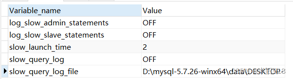
restart MySQL service , The implementation is as follows sql, Will long_query_time Restore to the default 10s, No more auditions .

SHOW VARIABLES LIKE '%long_query_time%';

4.5 Delete and restore slow query logs

After tuning, the slow query log can be deleted in time to save disk space . Of course, you can delete it manually .

rm DESKTOP-1PB99O1-slow.log

If deleted by mistake , And there is no backup or recycle bin , You can use the following command to restore the build .

# First, open the slow query log 
SET GLOBAL slow_query_log=ON;
# Recover slow query logs 
mysqladmin -u root -p flush-logs slow

5. see SQL Execution cost ：SHOW PROFILE

Check to see if it's on

show variables like 'profiling';

If it's not on , perform sql

mysql > set profiling = 'ON';

Use it .

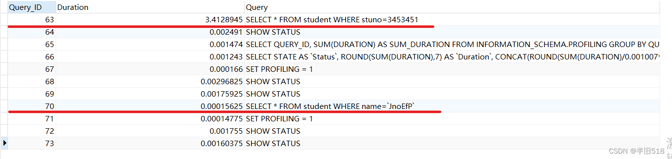
#  perform sql
SELECT * FROM student WHERE stuno=3453451;
SELECT * FROM student WHERE name=`JnoEfP`;
#  Analysis performance 
SHOW PROFILES;

Here the author has performed many in the current session sql 了 . The effect is as follows .

If you only need to view the latest one sql Performance details .

SHOW PROFILE;

The results are as follows .

You can view the specified sql Specified details of .

show profile cpu,block io for query 70;

If you find one sql The reason for the slowness is that the execution is slow (executing Fields are time consuming ), You can continue to use Explain Analyze specific sql Sentences .

Add :
show profile Common query parameters of ：
① ALL： Show all overhead information .
② BLOCK IO： Display block IO expenses .
③ CONTEXT SWITCHES： Context switching overhead .
④ CPU： Show CPU Overhead information .
⑤ IPC： Show send and receive overhead information .
⑥ MEMORY： Display memory overhead information .
⑦ PAGE FAULTS： Display page error overhead information .
⑧ SOURCE： Display and Source_function,Source_file,Source_line Related expense information .
⑨ SWAPS： Shows the number of exchanges overhead information .

in addition , In daily development , If in show profile In the query results of , Any of the following appears .sql Statements need to be optimized .

sql Statements need to be optimized ：
Coverting Heap to MyISAM： Query result is too large , There's no memory , Migrating to disk
Creating tmp table: Create a temporary table , Copy the data to the temporary table first , Delete the temporary table after use
Coping to tmp table on disk: Copy temporary data to disk , alert ！
locked.

Last , Attention is also needed ：SHOW PROFILE Command will be deprecated , But we can start from information_schema Medium profiling View the data table .

6. Analyze query statements ：EXPLAIN( a key )

6.1 EXPLAIN brief introduction

1️⃣ effect

Slow positioning sql after , have access to Describe perhaps Explain Conduct targeted analysis .

If you want to know SQL Implementation plan of , For example, a full table scan , Or index scan , Can pass EXPLAIN To complete .EXPLAIN Commands are the main way to see how the optimizer decides to execute the query . It can help us understand MySQL The overhead based optimizer , You can also get a lot of details about the access policies that may be considered by the optimizer , And when running SQL Which strategy is expected to be adopted by the optimizer at statement time .

2️⃣ website

5.7 edition mysql
8.0 edition mysql

3️⃣ Version Description

(1)MySQL 5.6.3 Before, I could only EXPLAIN SELECT;MYSQL 5.6.3 In the future EXPLAIN SELECT,EXPLAIN UPDATE,EXPLAIN DELETE
Be careful ,EXPLAIN Just look at the execution plan , Will not actually execute sql.

EXPLAIN DELETE FROM student_info WHERE id = 2;

SELECT * FROM student_info LIMIT 10;

Search above sql The results are as follows .id by 2 The data is still there .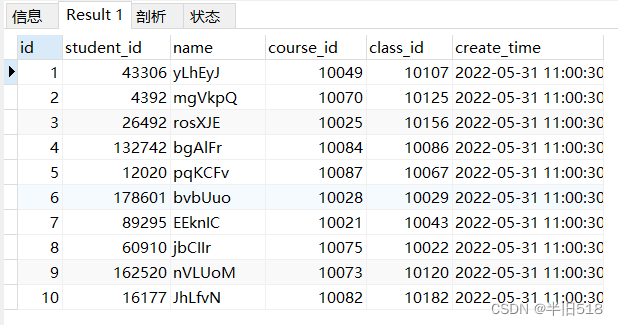

(2) stay 5.7 In previous versions , Want to display partition parameters partitions Need to use explain partitions command ; Want to show filtered Need to use explain extended command . stay 5.7 After version , Default explain Direct display partitions and filtered Information in ( Here's the picture ).

6.2 Basic grammar

First look at the list of parameters displayed . We will introduce them one by one later .

6.3 Data preparation

1️⃣. Build table

Create two tables to facilitate joint query

CREATE TABLE s1 (
	 id INT AUTO_INCREMENT,
	 key1 VARCHAR(100),
	 key2 INT,
	 key3 VARCHAR(100),
	 key_part1 VARCHAR(100),
	 key_part2 VARCHAR(100),
	 key_part3 VARCHAR(100),
	 common_field VARCHAR(100),
	  PRIMARY KEY (id),
	  INDEX idx_key1 (key1),
	  UNIQUE INDEX idx_key2 (key2),
	  INDEX idx_key3 (key3),
	  INDEX idx_key_part(key_part1, key_part2, key_part3)
) ENGINE=INNODB CHARSET=utf8;

CREATE TABLE s2 (
	 id INT AUTO_INCREMENT,
	 key1 VARCHAR(100),
	 key2 INT,
	 key3 VARCHAR(100),
	 key_part1 VARCHAR(100),
	 key_part2 VARCHAR(100),
	 key_part3 VARCHAR(100),
	 common_field VARCHAR(100),
	  PRIMARY KEY (id),
	  INDEX idx_key1 (key1),
	  UNIQUE INDEX idx_key2 (key2),
	  INDEX idx_key3 (key3),
	  INDEX idx_key_part(key_part1, key_part2, key_part3)
) ENGINE=INNODB CHARSET=utf8;

2️⃣ Create a storage function

DELIMITER //
CREATE FUNCTION rand_string1(n INT)
	RETURNS VARCHAR(255) # This function returns a string 
BEGIN
DECLARE chars_str VARCHAR(100) DEFAULT 'abcdefghijklmnopqrstuvwxyzABCDEFJHIJKLMNOPQRSTUVWXYZ';
	DECLARE return_str VARCHAR(255) DEFAULT '';
	DECLARE i INT DEFAULT 0;
	WHILE i < n DO
		SET return_str =CONCAT(return_str,SUBSTRING(chars_str,FLOOR(1+RAND()*52),1));
		SET i = i + 1;
	END WHILE;
	RETURN return_str;
END //
DELIMITER ;

Create a function , If it's wrong , You need to set parameters log_bin_trust_function_creators, Allows you to create function settings

set global log_bin_trust_function_creators=1;   #  No addition global Only the current window is valid .

3️⃣ Create stored procedure

To create s1 A stored procedure that inserts data into a table ：

DELIMITER //
CREATE PROCEDURE insert_s1 (IN min_num INT (10),IN max_num INT (10))
BEGIN
	DECLARE i INT DEFAULT 0;
	SET autocommit = 0;
	REPEAT
	SET i = i + 1;
	INSERT INTO s1 VALUES(
	 (min_num + i),
	 rand_string1(6),
	 (min_num + 30 * i + 5),
	 rand_string1(6),
	 rand_string1(10),
	 rand_string1(5),
	 rand_string1(10),
	 rand_string1(10));
	UNTIL i = max_num
	END REPEAT;
	COMMIT;
END //
DELIMITER ;

To create s2 A stored procedure that inserts data into a table ：

DELIMITER //
CREATE PROCEDURE insert_s2 (IN min_num INT (10),IN max_num INT (10))
BEGIN
	DECLARE i INT DEFAULT 0;
	SET autocommit = 0;
	REPEAT
	SET i = i + 1;
	INSERT INTO s2 VALUES((min_num + i),
		rand_string1(6),
		(min_num + 30 * i + 5),
		rand_string1(6),
		rand_string1(10),
		rand_string1(5),
		rand_string1(10),
		rand_string1(10));
	UNTIL i = max_num
	END REPEAT;
	COMMIT;
END //
DELIMITER ;

4️⃣ Calling stored procedure

s1 Addition of table data ： Join in 1 Ten thousand records ：

CALL insert_s1(10001,10000);

s2 Addition of table data ： Join in 1 Ten thousand records ：

CALL insert_s2(10001,10000);

6.4 EXPLAIN Action of each column

1️⃣ table

No matter how complex our query statement is , inside How many tables are included , In the end, each table needs to be Single table access Of , therefore MySQL Regulations EXPLAIN Each record output by the statement corresponds to the access method of a single table , Of this record table The column represents the table name of the table （ Sometimes it's not a real name , It may be abbreviated as ）.

EXPLAIN SELECT * FROM s1 INNER JOIN s2;

Here's the picture , A table corresponds to a record . notes ： Temporary tables also have corresponding records .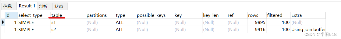

2️⃣id

Identification of a query . The results of the above query , Two records seem id All are 1. Why is that ？

actually , One SELECT Keyword corresponds to a id. below sql There are two select( Subquery ).

EXPLAIN SELECT * FROM s1 WHERE key1 IN (SELECT key1 FROM s2) OR key3 = 'a';

There are two different id yo . In fact, there is one in a query id Express .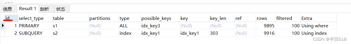

however , There's a pit here . Look at the following sentence .

EXPLAIN SELECT * FROM s1 WHERE key1 IN (SELECT key2 FROM s2 WHERE common_field = 'a');

Of two records id All are 1, Whether the little eyes are full of big doubts ？

This is because the optimizer will do the above sql Statement optimization , Convert it to a multi table join , Instead of subqueries . Because the subquery is actually a nested query , The time complexity is zero O(n^m), among m Is the number of nested layers , The time complexity of multi table query is O(n*m). In the above statement, the two queries do not need to have dependencies .

I want to see others Union Joint queries .

EXPLAIN SELECT * FROM s1 UNION SELECT * FROM s2;

So it turns out .

This is because Union Is the union of tables , You need to create a temporary table to remove duplicates , So there are three records . You can see the third record Extra It is a temporary table . A temporary table id yes Null.

I want to see others Union ALL.

EXPLAIN SELECT * FROM s1  UNION ALL SELECT * FROM s2;

Generate two records , Because it won't lose weight .

Summary
1.id If the same , It can be thought of as a group , From top to bottom
2. In all groups ,id The bigger the value is. , The higher the priority , Execute first
3. concerns ：id Number, each number , Represents an independent query , One sql The fewer query times, the better

3️⃣select_type

One sql There may be multiple queries in the statement . Every select Every small query has a select_type, Indicates what role it plays in large queries .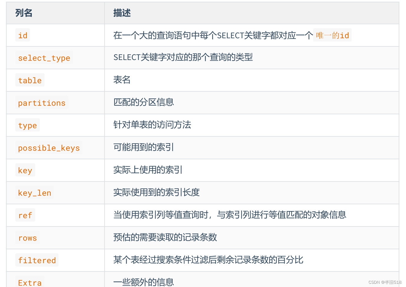

Let's start with a simple query .

EXPLAIN SELECT * FROM s1;

select_type yes simple

Look at the connection query .

EXPLAIN SELECT * FROM s1 INNER JOIN s2

still simple

Union The joint query . The query on the left is Primary, The query type on the right is Union, The query type of the de duplication temporary table is Union Result.

EXPLAIN SELECT * FROM s1 UNION SELECT * FROM s2;

Union All.

EXPLAIN SELECT * FROM s1  UNION ALL SELECT * FROM s2;

Don't explain .

Subquery , If it cannot be converted to the form of multi table connection , That is, it will not be automatically optimized by the optimizer . And the subquery is an unrelated subquery .

 EXPLAIN SELECT * FROM s1 WHERE key1 IN (SELECT key1 FROM s2) OR key3 = 'a';

The previous query , That is, the outer query is Primary, The inner query is SUBQUERY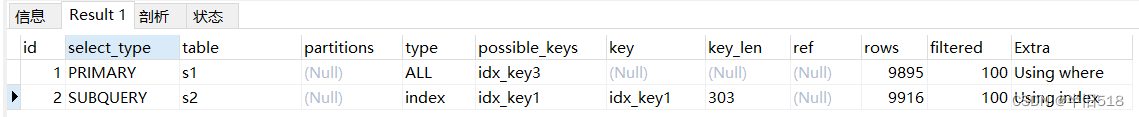

Subquery , If it cannot be converted to the form of multi table connection , And the subquery is a related subquery . For example, the following query uses external tables in the internal sub query .

EXPLAIN SELECT * FROM s1 WHERE key1 IN (SELECT key1 FROM s2 WHERE s1.key2 = s2.key2) OR key3 = 'a';

The outer query is Primary, The inner query is DEPENDENT SUBQUERY

It should be noted that DEPENDENT SUBQUERY The query statement of may be executed multiple times , Because memory queries depend on outer layer queries , So it may be that the outer layer passes a value , The inner layer executes the mode once .

Include in Union perhaps Union All Subquery of sql in , If each small query depends on an external query , Well, except for the leftmost query , The types of each small query are DEPENDENT UNION Oh .

EXPLAIN SELECT * FROM s1 WHERE key1 IN (SELECT key1 FROM s2 WHERE key1 = 'a' UNION SELECT key1 FROM s1 WHERE key1 = 'b');

The external query is Primary, The leftmost subquery is DEPENDENT SUBQUERY, The following subquery is DEPENDENT UNION, The type of temporary de duplication table is Union Result. Here you may be confused , No dependencies are found in the first subquery s1 ah . In fact, the optimizer will optimize at execution time , take IN Change to Exist, And move the external table to the internal table . Here, we just need to know , There will be articles to introduce the optimizer in the future .

also , For subqueries about derived tables .

EXPLAIN SELECT * FROM (SELECT key1, count(*) as c FROM s1 GROUP BY key1) AS derived_s1 where c > 1;

Its query type DERIVED.

When the optimizer executes the subquery, it chooses to optimize the subquery into a materialized table , When performing a join query with an outer query .

EXPLAIN SELECT * FROM s1 WHERE key1 IN (SELECT key1 FROM s2);

Look from the bottom up , The query type of the subquery is MATERIALIZED; The physicochemical process is based on id by 2 The query result table of , Its table yes subquery 2, The query type is SIMPLE, The outer layer is also equivalent to querying with fixed direct values , Its type is also SIMPLE.

The above introductions are all basic information , I haven't really introduced the index related information yet . Do you feel dizzy , Let's use a table to summarize .

4️⃣partitions ( Can be omitted )

If you want to know more about it , You can test . Create a partition table ：

--  Create a partition table ,
--  according to id Partition ,id<100 p0 Partition , other p1 Partition 
CREATE TABLE user_partitions (id INT auto_increment,
	NAME VARCHAR(12),PRIMARY KEY(id))
  	PARTITION BY RANGE(id)(
    PARTITION p0 VALUES less than(100),
    PARTITION p1 VALUES less than MAXVALUE
 );

Inquire about id Greater than 200（200>100,p1 Partition ） The record of

DESC SELECT * FROM user_partitions WHERE id>200;

View execution plan ,partitions yes p1, Comply with our zoning rules

5️⃣type *

type Indicates that when a query is executed, it is for mysql How to access a table in . This is an important indicator , Indicates how we access and obtain data .

The complete access method is as follows ： system , const , eq_ref , ref , fulltext , ref_or_null ,index_merge , unique_subquery , index_subquery , range , index , ALL.

The following will explain in detail .

(1)system

When there is only one record in the table , And the engine statistics stored in this table are accurate , such as MYISAM,Memory, The access method is System. This approach is almost the highest performance , Of course we hardly use it .

CREATE TABLE t(i int) Engine=MyISAM;
INSERT INTO t VALUES(1);
EXPLAIN SELECT * FROM t;

The query results are as follows .

Whenever we insert another piece of data .

INSERT INTO t VALUES(2);
EXPLAIN SELECT * FROM t;

The access method becomes the worst performance full table scan ALL.

If the storage engine is InnoDB, Even if there is only one piece of data , Its access mode is also ALL, This is because InnnoDB Accessing data is not precise .

(2)Const

When we use a primary key or a unique headset index , When matching equivalently with a constant , The way to access a single table is const. This access method is less efficient than system, But it is also very efficient .

For example, match the primary key with the constant , Perform equivalent query .

EXPLAIN SELECT * FROM s1 WHERE id = 10005;

For example, yes. Unique Unique secondary index of the identifier key2 Match with constant , Perform equivalent query .

EXPLAIN SELECT * FROM s1 WHERE key2 = 10066;

（4）eq_ref

Proceed again Link query when , If Was the driver table The query is performed by matching the primary key or the unique secondary index , The access method of the driven table is eq_ref. This is also a very good performance way .

EXPLAIN SELECT * FROM s1 INNER JOIN s2 ON s1.id = s2.id;

The above connection query statement , For driving tables , That's right s1 Scan the whole table , Find eligible data , Therefore, its type yes All, For driven tables , Equivalent query is performed on the data queried from the driver table , So its access method is eq_ref.

（5）ref

When using ordinary secondary indexes to match constants equivalently ,type yes ref.

EXPLAIN SELECT * FROM s1 WHERE key1 = 'a';

give the result as follows .

Let's test you . following sql What is the reference type of ？

EXPLAIN SELECT * FROM s1 WHERE key3 = 10066;

Look at the answer . Did you guess wrong . yes All. This is because key3 The field of is varchar type , But the constant value here is an integer , So you need to use functions for implicit type conversions , Once you use the function , The index fails , So the access type becomes a full table scan All

We use the types of pairs for constants .

EXPLAIN SELECT * FROM s1 WHERE key3 = '10066';

It is expected ref Access type .

（6）ref_or_null

When using ordinary secondary index for equivalence matching , When the index value can be Null when ,type yes ref_or_null.

EXPLAIN SELECT * FROM s1 WHERE key1 = 'a' OR key1 IS NULL;

give the result as follows .

（7）index_merge

When accessing a single table , If a single column index is established for multiple query fields , Use OR Connect , Its access type is index_merge.

 EXPLAIN SELECT * FROM s1 WHERE key1 = 'a' OR key3 = 'a';

The result is as follows . At the same time, you can see key This field , Two indexes are used .

Guess the following sql The type of reference

 EXPLAIN SELECT * FROM s1 WHERE key1 = 'a' AND key3 = 'a';

Are you right ？ The answer is ref, This is because of the use of AND When connecting two queries , In fact, only key1 The index of .

(8)unique_subquery

For some containing IN Of subcase, If the optimizer decides to IN The subquery optimization is EXIST Subquery , And the sub query can use the primary key for equivalent matching , The execution plan of the subquery type Namely unique_subquery.

EXPLAIN SELECT * FROM s1 WHERE key2 IN (SELECT id FROM s2 where s1.key1 = s2.key1) OR key3 = 'a';

give the result as follows .

(9)range

The type of access plan for range lookup is range.

EXPLAIN SELECT * FROM s1 WHERE key1 IN ('a', 'b', 'c');

(10)index

When we can use Index overlay , But when you need to scan all the index records , The access method of this table is index. Index coverage will be described in detail when the optimizer is introduced in the following article , For your understanding , First, a brief introduction is as follows . For example, below sql In the sentence ,key_part2 ,key_part2 All belong to the union index INDEX idx_key_part(key_part1, key_part2, key_part3) Part of , This union index can be used to find data , It is not necessary to perform a table return operation , In this case, even if the index covers .

EXPLAIN SELECT key_part2 FROM s1 WHERE key_part2 = 'a';

give the result as follows .

(11)ALL

EXPLAIN SELECT * FROM s1;

result

reminder ： Many friends here feel that they can't remember , In fact, you can collect this blog , perform EXPLAIN Time corresponds to the result , Reverse search the corresponding content of the blog , After all, we just need to be able to read the results of performance analysis .

Finally, let's make a summary .

The result value from the best to the worst is ： system > const > eq_ref > ref > fulltext > ref_or_null > index_merge > unique_subquery > index_subquery > range > index > ALL Some of the more important ones are extracted （ See the bold section ）.
SQL Objectives of performance optimization ： At the very least range Level , The requirement is ref Level , It is best to consts Level .（ Alibaba development manual requirements ）

6️⃣possible_keys and key

Indicates the index that may be used and the index that is actually used .

EXPLAIN SELECT * FROM s1 WHERE key1 > 'z' AND key3 = 'a';

For the optimizer , elective possible_keys The less, the better. , Because there are more options , It takes more time to filter . in addition , The optimizer will evaluate the efficiency of querying each index , So as to select the actual key. And because the optimizer will sql To optimize , It is entirely possible that possible_keys yes null, however key Not for null The situation of .

7️⃣key_len *

The length of the index actually used , Unit is byte . It can help you check whether you make full use of the index , It mainly has certain reference for the joint index , For the same index ,key_len The higher the value, the better ( Compare with yourself , It will be explained later ).

mysql> EXPLAIN SELECT * FROM s1 WHERE id = 10005;

The result is as follows , yes 4, How did this result come out ？

This is because the primary key is used id As index , The type is int, Occupy 4 Bytes .

Come again . Guess the following key_len How much is the .

 EXPLAIN SELECT * FROM s1 WHERE key2 = 10126;

what ？ Your guess is 4, Then you have to give me one button triple . Because the answer is 5.

This is because although key2 It's also int type , But it was unique modification , No identification is not empty ( The primary keys are all non empty ), So add the upper value mark , Is the total 5 Bytes , If you can't understand it, you can read this supplementary lesson ：Mysql Advanced index 02——InnoDB The data storage structure of storage engine

Come again .

 EXPLAIN SELECT * FROM s1 WHERE key1 = 'a';

The answer is 303, Because the type is varchar(100),100 Characters ,utf-8 Each character takes 3 Bytes , common 300 Bytes , Add the variable length list 2 Bytes and a null identifier occupy one byte , common 303 byte .

Look at the union index .

EXPLAIN SELECT * FROM s1 WHERE key_part1 = 'a';

Its key_len still 303, There's no need to explain .

Take a look at the following joint index .

 EXPLAIN SELECT * FROM s1 WHERE key_part1 = 'a' AND key_part2 = 'b';

As a result, 606 Oh .

This query is key-len Larger than the above query , The performance is better than the above , How do you understand that ？ In fact, as long as you read my previous Introduction B+ The tree article is easy to understand . Because in the table of contents, I have to consider key_part1 , And think about key_part12, The located data is more accurate , Smaller range , Need to load I/O The number of data pages will be less , Is the performance better .

I also post blog links to you :MySql Advanced index 01—— Explain the data structure of the index in depth ：B+ Trees
, Don't you pay attention to such a good blogger ？

Guess the following sql After execution key_len How much is the

	EXPLAIN SELECT * FROM s1 WHERE key_part3 = 'a';

It's empty , Because we don't use indexes , This is what we have been talking about Leftmost prefix principle , It will be described in detail later .

practice ：key_len The length formula of ：
varchar(10) Variable length field and allow NULL = 10 * ( character set：utf8=3,gbk=2,latin1=1)+1(NULL)+2( Variable length field )
varchar(10) Variable length field and not allowed NULL = 10 * ( character set：utf8=3,gbk=2,latin1=1)+2( Variable length field )
char(10) Fixed field and allow NULL = 10 * ( character set：utf8=3,gbk=2,latin1=1)+1(NULL)
char(10) Fixed field and not allowed NULL = 10 * ( character set：utf8=3,gbk=2,latin1=1)

8️⃣.ref

When an index column performs an equivalent query , Object information matching the index column .

Match with constant equivalence .

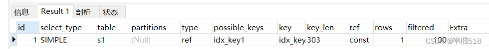
EXPLAIN SELECT * FROM s1 WHERE key1 = 'a';

Its ref yes const

Come again . Connection query .

EXPLAIN SELECT * FROM s1 INNER JOIN s2 ON s1.id = s2.id;

For driven tables s2 The executed query references atguigudb1.s1.id Field for equivalent query .

Finally, let's look at the use of functions . Its ref Namely func.

 EXPLAIN SELECT * FROM s1 INNER JOIN s2 ON s2.key1 = UPPER(s1.key1);

9️⃣ rows *

Estimated number of log entries to read . The smaller the number of entries, the better . This is because the smaller the value , load I/O The fewer pages you have .

EXPLAIN SELECT * FROM s1 WHERE key1 > 'z';

result .

1️⃣0️⃣filtered

The percentage of the remaining records filtered after the search criteria . The higher the percentage, the better , Like the same rows yes 40, If filter yes 100, It is from 40 Search in records , If filter yes 10, It is from 400 Search in records , In comparison, of course, the former is more efficient .

If a single table scan is performed , When calculating, you need to estimate how many records other than the corresponding search criteria meet . If you feel dizzy, take a look at the following example .

EXPLAIN SELECT * FROM s1 WHERE key1 > 'z' AND common_field = 'a';

The result is 10, Express 398 Records meet key1 > 'z’ Conditions , this 398 Bar record 10% Satisfy common_field = 'a’ Conditions .

actually , For single table query , This field doesn't make much sense , We pay more attention to the connection query filtered value , It determines the number of times the driven table is to be executed .

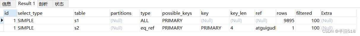
EXPLAIN SELECT * FROM s1 INNER JOIN s2 ON s1.key1 = s2.key1 WHERE
s1.common_field = 'a';

give the result as follows . Mark the drive table s1 The number of records provided to the driven table is 9895 strip , among 989.5 The filter conditions are met s1.key1 = s2.key1, Then the driven table needs to execute 990 Queries .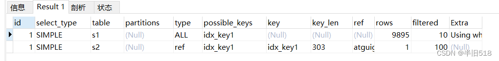

1️⃣1️⃣ Extra *

Provide some additional information , Can be more accurate to know MySQL How to execute a given query statement .
No tables used, Don't explain .

EXPLAIN SELECT 1;

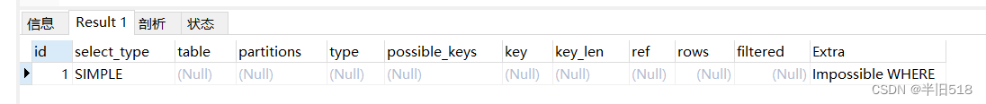
Impossible WHERE, When the query condition can never be satisfied , This message appears when no data can be found .

 EXPLAIN SELECT * FROM s1 WHERE 1 != 1;

Using where, Index not used , ordinary where Inquire about

EXPLAIN SELECT * FROM s1 WHERE common_field = 'a';

Use index query , Use the index silently , There is no additional information .

EXPLAIN SELECT * FROM s1 WHERE key1 = 'a';

Index plus normal where, Then still using where

EXPLAIN SELECT * FROM s1 WHERE key1 = 'a' AND common_field = 'a'

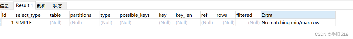
No matching min/max row. When there is MIN、MAX Wait for the aggregate function , But it doesn't meet where The search record of the condition , Will provide additional information No matching min/max row.( There is no satisfaction in the table where Conditional words , look for min、max It makes no sense )

EXPLAIN SELECT MIN(key1) FROM s1 WHERE key1 = 'abcdefg';

Select tables optimized away, When there is MIN、MAX Wait for the aggregate function , Yes where The search record of the condition .

EXPLAIN SELECT MIN(key1) FROM s1 WHERE key1 = 'vTilEo';

Using index, When using the overlay index, you will be prompted . The so-called overlay index , The index covers all the fields to be queried , There is no need to use cluster index for back table lookup , Take the following example , Use key1 As a search condition , This field is indexed ,B+ The tree can find key1 Fields and primary keys , So just look for key1 Fields do not need to be returned to the table , This is a very good situation .

`EXPLAIN SELECT key1 FROM s1 WHERE key1 = 'a';

Using index condition： Although the index column appears in the search column , But you can't use indexes , It's a hole .

For example, although the following query has index columns as query criteria , However, you still need to perform a back table lookup , The back table operation is a random operation I/O, More time-consuming .

EXPLAIN SELECT * FROM s1 WHERE key1 > 'z' AND key1 LIKE '%a';

In the above case, you can use Index push down ( You can configure through configuration items ), Make us use WHERE key1 > ‘z’ The obtained results are fuzzy matched first key1 LIKE ‘%a’, Then go back to your watch , You can reduce the number of times to return to the table .

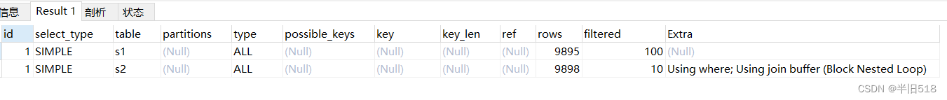
Using join buffer (Block Nested Loop)： In connection queries , When the driven table can not effectively use the index to improve the speed , The database uses caching to improve performance as much as possible .

EXPLAIN SELECT * FROM s1 INNER JOIN s2 ON s1.common_field = s2.common_field;

Not exists: When using the left outer connection , When the search condition of the driven table requires a field to be null, And this field is not empty , Will prompt .

EXPLAIN SELECT * FROM s1 LEFT JOIN s2 ON s1.key1 = s2.key1 WHERE s2.id IS NULL;

Using intersect(…) 、 Using union(…) and Using sort_union(…): Index merging .

EXPLAIN SELECT * FROM s1 WHERE key1 = 'a' OR key3 = 'a';

Zero limit

EXPLAIN SELECT * FROM s1 LIMIT 0;

Using filesort： The index cannot be used for sorting , Only in memory ( Fewer records ) Or on disk ( There are many records ) Sort , This situation is tragic .

EXPLAIN SELECT * FROM s1 ORDER BY common_field LIMIT 10;

Using temporary: Common field de duplication 、 grouping , Index not available , Use a temporary watch , This also needs to be optimized .

EXPLAIN SELECT DISTINCT common_field FROM s1;

Add
EXPLAIN Don't think about all kinds of Cache
EXPLAIN Can't show MySQL Optimizations done when executing queries
EXPLAIN I won't tell you about triggers 、 The impact of stored procedure information or user-defined functions on the query is estimated , Not exactly

7.EXPLAIN Further use of

7.1、EXPLAIN Four output formats

Here to talk EXPLAIN The output format of .EXPLAIN You can output four formats ： Traditional format ,JSON Format , TREE Format as well as Visual output . Users can choose their own format according to their needs .

1️⃣ Traditional format

The traditional format is simple and clear , The output is a tabular form , Outline query plan .

EXPLAIN  SELECT s1.key1, s2.key1 FROM s1 LEFT JOIN s2 ON s1.key1 = s2.key1 WHERE s2.common_field IS NOT NULL;

2️⃣JSON Format

stay EXPLAIN Add... Between the word and the real query statement FORMAT=JSON .
Traditional format and json The fields of the format have corresponding relationships as shown in the following table (mysql5.7 Official documents ).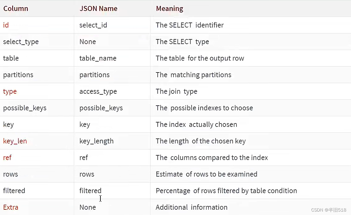

demo as follows .

EXPLAIN FORMAT=JSON SELECT s1.key1, s2.key1 FROM s1 LEFT JOIN s2 ON s1.key1 = s2.key1 WHERE s2.common_field IS NOT NULL;

give the result as follows . You can see json The information content of the format will be richer . In especial cost Information , It is an important indicator to measure the quality of an implementation plan .

{
  "query_block": {
    "select_id": 1,
    "cost_info": {
      "query_cost": "12766.44"
    },
    "nested_loop": [
      {
        "table": {
          "table_name": "s2",
          "access_type": "ALL",
          "possible_keys": [
            "idx_key1"
          ],
          "rows_examined_per_scan": 9898,
          "rows_produced_per_join": 8908,
          "filtered": "90.00",
          "cost_info": {
            "read_cost": "294.96",
            "eval_cost": "1781.64",
            "prefix_cost": "2076.60",
            "data_read_per_join": "15M"
          },
          "used_columns": [
            "key1",
            "common_field"
          ],
          "attached_condition": "((`atguigudb1`.`s2`.`common_field` is not null) and (`atguigudb1`.`s2`.`key1` is not null))"
        }
      },
      {
        "table": {
          "table_name": "s1",
          "access_type": "ref",
          "possible_keys": [
            "idx_key1"
          ],
          "key": "idx_key1",
          "used_key_parts": [
            "key1"
          ],
          "key_length": "303",
          "ref": [
            "atguigudb1.s2.key1"
          ],
          "rows_examined_per_scan": 1,
          "rows_produced_per_join": 8908,
          "filtered": "100.00",
          "using_index": true,
          "cost_info": {
            "read_cost": "8908.20",
            "eval_cost": "1781.64",
            "prefix_cost": "12766.44",
            "data_read_per_join": "15M"
          },
          "used_columns": [
            "key1"
          ]
        }
      }
    ]
  }
}

You may have questions “cost_info” The cost inside looks strange , How are they calculated ？

First look at s1 Tabular "cost_info" part ：

"cost_info": {
  "read_cost": "1840.84",
  "eval_cost": "193.76",
  "prefix_cost": "2034.60",
  "data_read_per_join": "1M"
}

read_cost It's made up of the two parts below ：

• IO cost
• testing rows × (1 - filter) Bar record CPU cost

rows and filter All of them are the output columns of our previous introduction to the implementation plan , stay JSON Format of the implementation plan ,rows amount to rows_examined_per_scan,filtered The name does not change

eval_cost This is how it is calculated ：

• testing rows × filter Cost of records .

prefix_cost It's a separate query s1 Cost of tables , That is to say ：read_cost + eval_cost
data_read_per_join Represents the amount of data to be read in this query .

about s2 Tabular “cost_info” Part of it is like this ：

"cost_info": {
  "read_cost": "968.80",
  "eval_cost": "193.76",
  "prefix_cost": "3197.16",
  "data_read_per_join": "1M"
}

because s2 A table is a driven table , So it can be read many times , there read_cost and eval_cost It's a visit many times s2 The cumulative value at the end of the table , We are mainly concerned about the prefix_cost The value of represents the estimated cost of the entire join query , It's a single query s1 Tables and multiple queries s2 The sum of the cost after the table , That is to say ：

968.80 + 193.76 + 2034.60 = 3197.16

3️⃣TREE Format

TREE The format is 8.0.16 New format introduced after version , Mainly based on the query The relationship between the parts and Execution sequence of each part To describe how to query .

 EXPLAIN FORMAT=tree SELECT * FROM s1 INNER JOIN s2 ON s1.key1 = s2.key2 WHERE
s1.common_field = 'a'\G
*************************** 1. row ***************************
EXPLAIN: -> Nested loop inner join (cost=1360.08 rows=990)
 -> Filter: ((s1.common_field = 'a') and (s1.key1 is not null)) (cost=1013.75
rows=990)
   -> Table scan on s1 (cost=1013.75 rows=9895)
 -> Single-row index lookup on s2 using idx_key2 (key2=s1.key1), with index
condition: (cast(s1.key1 as double) = cast(s2.key2 as double)) (cost=0.25 rows=1)
1 row in set, 1 warning (0.00 sec)

4️⃣ Visual output

Visual output , Can pass MySQL Workbench Visual view MySQL Implementation plan of . By clicking on Workbench Magnifying glass icon , You can generate a visual query plan .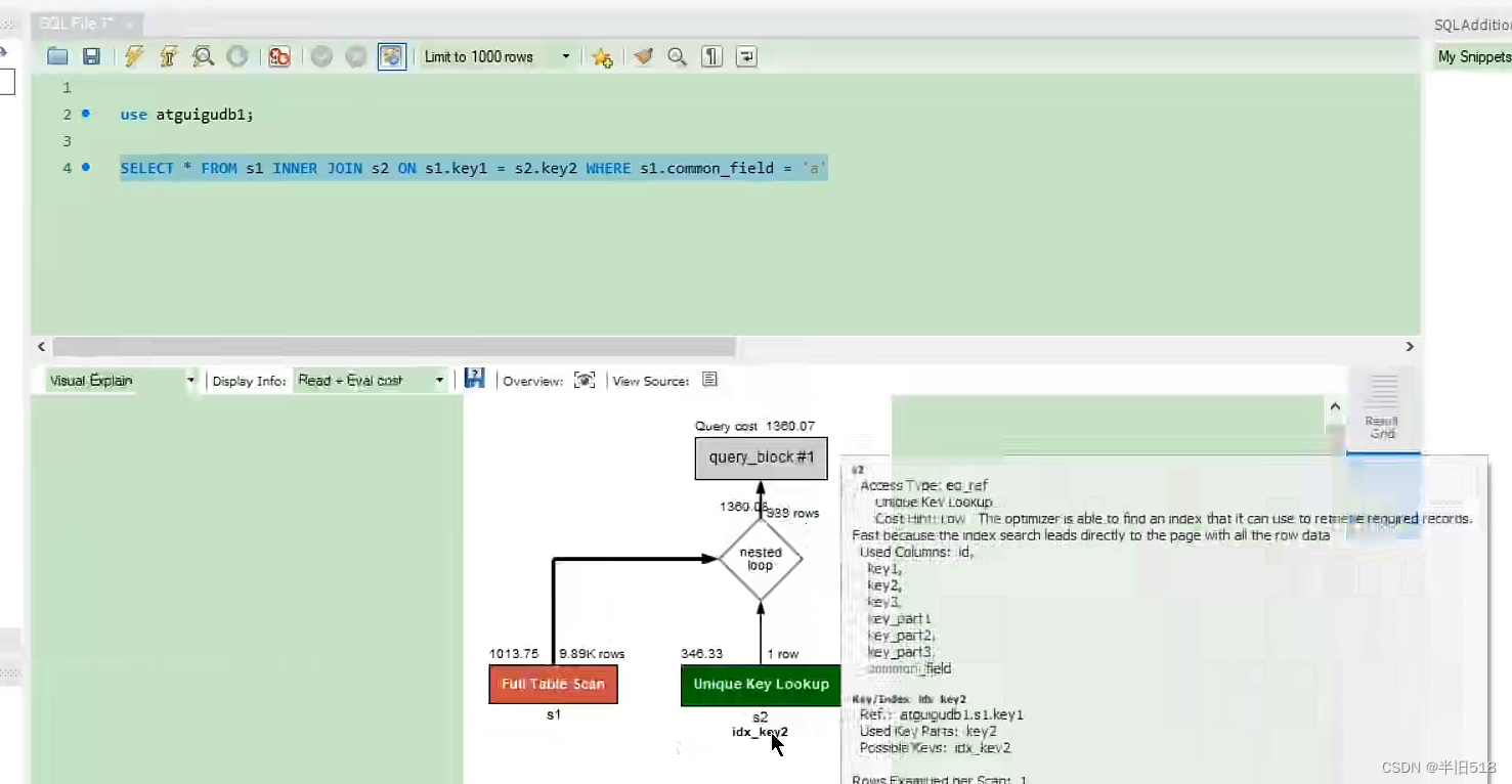

The figure above shows the table from left to right . A red box indicates Full table scan , The green box indicates the use of Index lookup
For each table , Show index used . Also note that , Above each table's box is an estimate of the number of rows found for each table access and the cost of accessing that table .

7.2 SHOW WARNINGS Use

You can display what the database actually does sql

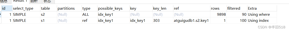
First use Explain, We wrote sql It is reasonable to use s1 As a driving table

 EXPLAIN SELECT s1.key1, s2.key1 FROM s1 LEFT JOIN s2 ON s1.key1 = s2.key1 WHERE s2.common_field IS NOT NULL;

The result of execution is s2 As a driver table ,s1 As a driven table

Then use SHOW WARNINGS

mysql> SHOW WARNINGS\G
*************************** 1. row ***************************
 Level: Note
 Code: 1003
Message: /* select#1 */ select `atguigu`.`s1`.`key1` AS `key1`,`atguigu`.`s2`.`key1`
AS `key1` from `atguigu`.`s1` join `atguigu`.`s2` where ((`atguigu`.`s1`.`key1` =
`atguigu`.`s2`.`key1`) and (`atguigu`.`s2`.`common_field` is not null))
1 row in set (0.00 sec)

above message Database optimization is shown in 、 After rewriting ‘ real ’ Executed query statements . Sure enough, it helped us optimize .

8. Analyze optimizer execution plan ：trace

OPTIMIZE_TRACE yes mysql5.6 A tracking tool introduced in , It can track various decisions made by the optimizer , For example, the method of accessing the table , Various overhead calculations , All kinds of transformations , The results will be recorded in information_schema.optimizer_trace in .

Turn on .

SET optimizer_trace="enabled=on",end_markers_in_json=on;
set optimizer_trace_max_mem_size=1000000;

After opening , The following statements can be analyzed ：

• SELECT
• INSERT
• REPLACE
• UPDATE
• DELETE
• EXPLAIN
• SET
• DECLARE
• CASE
• IF
• RETURN
• CALL

test ： The implementation is as follows SQL sentence

select * from student where id < 10;

Last , Inquire about information_schema.optimizer_trace We can know MySQL How to execute SQL Of

select * from information_schema.optimizer_trace\G

give the result as follows

*************************** 1. row ***************************
 // The first 1 part ： Query statement 
 QUERY: select * from student where id < 10
 // The first 2 part ：QUERY The tracking information of the statement corresponding to the field 
 TRACE: {
    
 "steps": [
 {
    
   "join_preparation": {
      // Preparatory work 
    "select#": 1,
    "steps": [
    {
    
      "expanded_query": "/* select#1 */ select `student`.`id` AS
`id`,`student`.`stuno` AS `stuno`,`student`.`name` AS `name`,`student`.`age` AS
`age`,`student`.`classId` AS `classId` from `student` where (`student`.`id` < 10)"
    }
   ] /* steps */
  } /* join_preparation */
 },
 {
    
   "join_optimization": {
      // To optimize 
    "select#": 1,
    "steps": [
    {
    
      "condition_processing": {
      // Conditional processing 
       "condition": "WHERE",
       "original_condition": "(`student`.`id` < 10)",
       "steps": [
       {
    
         "transformation": "equality_propagation",
         "resulting_condition": "(`student`.`id` < 10)"
       },
       {
    
         "transformation": "constant_propagation",
         "resulting_condition": "(`student`.`id` < 10)"
       },
       {
    
         "transformation": "trivial_condition_removal",
         "resulting_condition": "(`student`.`id` < 10)"
       }
] /* steps */
     } /* condition_processing */
    },
    {
    
      "substitute_generated_columns": {
      // Replace the generated column 
     } /* substitute_generated_columns */
    },
    {
    
      "table_dependencies": [   // Table dependencies 
      {
    
        "table": "`student`",
        "row_may_be_null": false,
        "map_bit": 0,
        "depends_on_map_bits": [
       ] /* depends_on_map_bits */
      }
     ] /* table_dependencies */
    },
    {
    
      "ref_optimizer_key_uses": [   // Use the key 
     ] /* ref_optimizer_key_uses */
    },
    {
    
      "rows_estimation": [   // Line judgment 
      {
    
        "table": "`student`",
        "range_analysis": {
    
         "table_scan": {
    
          "rows": 3973767,
          "cost": 408558
        } /* table_scan */,   // Scan table 
         "potential_range_indexes": [   // Potential range index 
         {
    
           "index": "PRIMARY",
           "usable": true,
           "key_parts": [
            "id"
          ] /* key_parts */
         }
        ] /* potential_range_indexes */,
         "setup_range_conditions": [   // Set range conditions 
        ] /* setup_range_conditions */,
         "group_index_range": {
    
          "chosen": false,
          "cause": "not_group_by_or_distinct"
        } /* group_index_range */,
         "skip_scan_range": {
    
          "potential_skip_scan_indexes": [
          {
    
            "index": "PRIMARY",
            "usable": false,
            "cause": "query_references_nonkey_column"
          }
         ] /* potential_skip_scan_indexes */
        } /* skip_scan_range */,
         "analyzing_range_alternatives": {
      // Analysis range options 
          "range_scan_alternatives": [
          {
    
"index": "PRIMARY",
            "ranges": [
             "id < 10"
           ] /* ranges */,
            "index_dives_for_eq_ranges": true,
            "rowid_ordered": true,
            "using_mrr": false,
            "index_only": false,
            "rows": 9,
            "cost": 1.91986,
            "chosen": true
          }
         ] /* range_scan_alternatives */,
          "analyzing_roworder_intersect": {
    
           "usable": false,
           "cause": "too_few_roworder_scans"
         } /* analyzing_roworder_intersect */
        } /* analyzing_range_alternatives */,
         "chosen_range_access_summary": {
       // Select the scope to access the summary 
          "range_access_plan": {
    
           "type": "range_scan",
           "index": "PRIMARY",
           "rows": 9,
           "ranges": [
            "id < 10"
          ] /* ranges */
         } /* range_access_plan */,
          "rows_for_plan": 9,
          "cost_for_plan": 1.91986,
          "chosen": true
        } /* chosen_range_access_summary */
       } /* range_analysis */
      }
     ] /* rows_estimation */
    },
    {
    
      "considered_execution_plans": [  // Consider implementation plan 
      {
    
        "plan_prefix": [
       ] /* plan_prefix */,
        "table": "`student`",
        "best_access_path": {
      // Best access path 
         "considered_access_paths": [
         {
    
           "rows_to_scan": 9,
           "access_type": "range",
           "range_details": {
    
            "used_index": "PRIMARY"
          } /* range_details */,
           "resulting_rows": 9,
           "cost": 2.81986,
           "chosen": true
         }
        ] /* considered_access_paths */
       } /* best_access_path */,
        "condition_filtering_pct": 100,  // Row filter percentage 
        "rows_for_plan": 9,
        "cost_for_plan": 2.81986,
        "chosen": true
      }
     ] /* considered_execution_plans */
    },
    {
    
      "attaching_conditions_to_tables": {
      // Attach the condition to the table 
       "original_condition": "(`student`.`id` < 10)",
       "attached_conditions_computation": [
      ] /* attached_conditions_computation */,
       "attached_conditions_summary": [  // Summary of additional conditions 
       {
    
         "table": "`student`",
         "attached": "(`student`.`id` < 10)"
       }
      ] /* attached_conditions_summary */
     } /* attaching_conditions_to_tables */
    },
    {
    
      "finalizing_table_conditions": [
      {
    
        "table": "`student`",
        "original_table_condition": "(`student`.`id` < 10)",
        "final_table_condition ": "(`student`.`id` < 10)"
      }
     ] /* finalizing_table_conditions */
    },
    {
    
      "refine_plan": [  // Streamline plans 
      {
    
        "table": "`student`"
      }
     ] /* refine_plan */
    }
   ] /* steps */
  } /* join_optimization */
 },
 {
    
   "join_execution": {
       // perform 
    "select#": 1,
    "steps": [
   ] /* steps */
  } /* join_execution */
 }
] /* steps */
}
// The first 3 part ： When the tracking information is too long , The number of bytes of truncated trace information .
MISSING_BYTES_BEYOND_MAX_MEM_SIZE: 0  // Missing bytes exceeding maximum capacity 
// The first 4 part ： Whether the user executing the trace statement has permission to view the object . When you don't have permission , The column information is 1 And TRACE Field is empty , Generally in 
 Call with SQL SECURITY DEFINER In the case of stored procedures , This problem will arise .
INSUFFICIENT_PRIVILEGES: 0  // Missing permissions 
1 row in set (0.00 sec)

9.MySQL Monitor analysis view -sys schema

9.1 Sys schema View summary

performace-schema and information-schema Can be used to analyze database performance ,mysql5.7 And designed -sys schema It integrates the above two schema, Also let them display as views , Easier to understand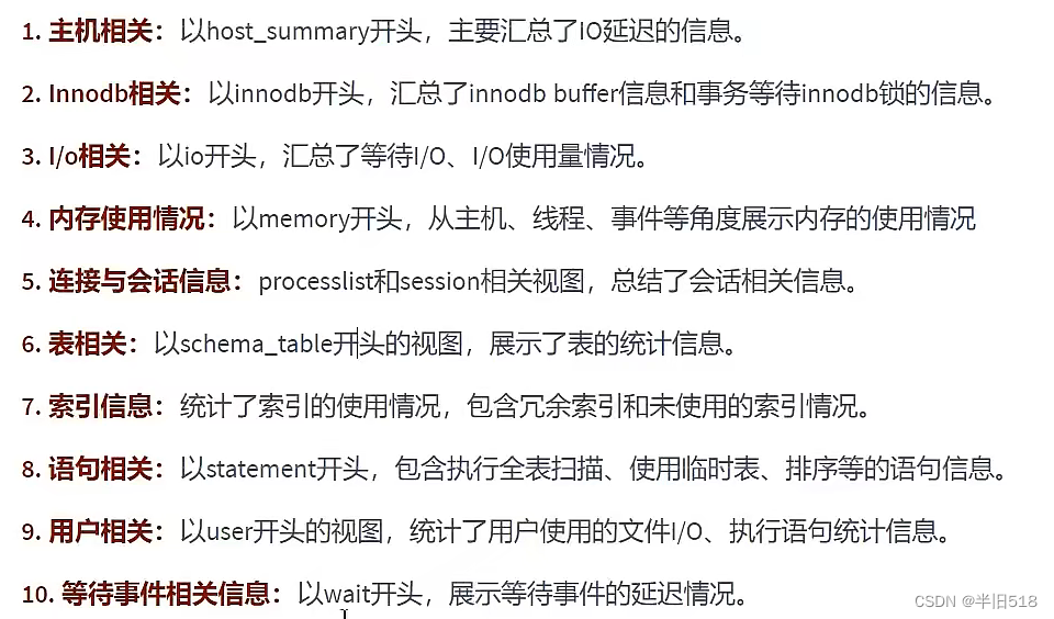

9.2 Sys schema View usage scenario

The index case

#1.  Query redundant index 
select * from sys.schema_redundant_indexes;

#2.  Query unused indexes 
select * from sys.schema_unused_indexes;

#3.  Query index usage 
select index_name,rows_selected,rows_inserted,rows_updated,rows_deleted
from sys.schema_index_statistics where table_schema='dbname' ;

Table related

# 1.  The number of visits to the query table 
select table_schema,table_name,sum(io_read_requests+io_write_requests) as io from sys.schema_table_statistics group by table_schema,table_name order by io desc;

# 2.  Query occupancy bufferpool More tables 
select object_schema,object_name,allocated,data
from sys.innodb_buffer_stats_by_table order by allocated limit 10;

# 3.  Check the full table scanning of the table 
select * from sys.statements_with_full_table_scans where db='dbname';

Statement related

#1.  monitor SQL Frequency of execution 
select db,exec_count,query from sys.statement_analysis
order by exec_count desc;

#2.  The monitoring uses sorted SQL
select db,exec_count,first_seen,last_seen,query
from sys.statements_with_sorting limit 1;

#3.  Monitor the use of temporary tables or disk temporary tables SQL
select db,exec_count,tmp_tables,tmp_disk_tables,query
from sys.statement_analysis where tmp_tables>0 or tmp_disk_tables >0
order by (tmp_tables+tmp_disk_tables) desc;

IO relevant

# View consumed disks IO The file of 
select file,avg_read,avg_write,avg_read+avg_write as avg_io
from sys.io_global_by_file_by_bytes order by avg_read  limit 10;

Innodb relevant

# Row lock blocking 
select * from sys.innodb_lock_waits;