吴恩达逻辑回归2

正则化逻辑回归

在这部分练习中，您将实现正则化逻辑回归
预测来自制造厂的微芯片是否通过质量保证

import numpy as np
import pandas as pd
import matplotlib.pyplot as plt

1. 数据可视化

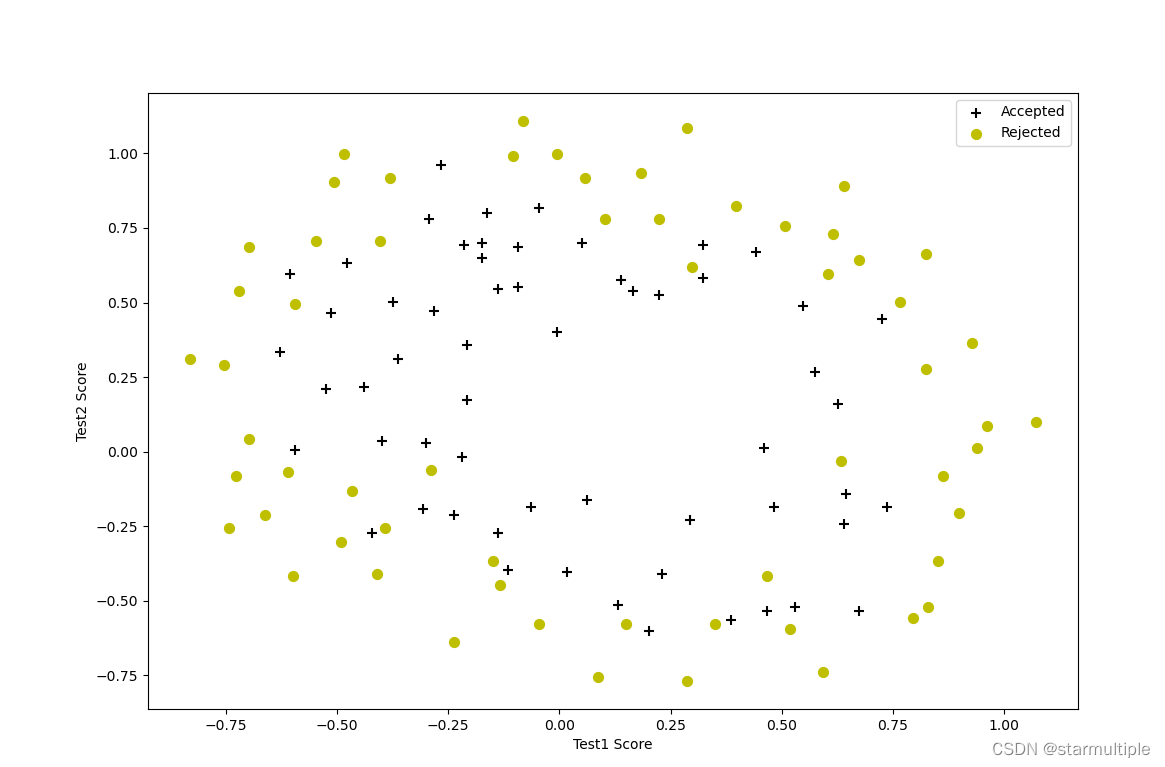
plotData 用于生成一个
如图 所示，其中轴是两个测试分数，而正（y = 1，接受）和否定（y = 0，拒绝）示例显示为不同的标记。

path = 'ex2data2.txt'
df = pd.read_csv(path, header=None, names=['Microchip Test1', 'Microchip Test2', 'Accepted'])
df.head()

df.describe()

pos = df[df['Accepted'].isin([1])]
neg = df[df['Accepted'].isin([0])]

fig, ax = plt.subplots(figsize=(12, 8))
ax.scatter(pos['Microchip Test1'], pos['Microchip Test2'], s=50, c='black', marker='+', label='Accepted')
ax.scatter(neg['Microchip Test1'], neg['Microchip Test2'], s=50, c='y', marker='o', label='Rejected')
ax.legend()
ax.set_xlabel('Test1 Score')
ax.set_ylabel('Test2 Score')
plt.show()

特征映射

更好地拟合数据的一种方法是从每个数据点创建更多特征。在提供的函数 mapFeature.m 中，我们将特征映射到 x 1 和 x 2 的所有多项式项，直到六次方。

def feature_mapping(x, y, power, as_ndarray=False):
    data = {
    'f{0}{1}'.format(i-p, p): np.power(x, i-p) * np.power(y, p)
                for i in range(0, power+1)
                for p in range(0, i+1)
           }
    if as_ndarray:
        return pd.DataFrame(data).values
    else:
        return pd.DataFrame(data)

x1 = df.Test1.values
x2 = df.Test2.values
Y = df.Accepted

data = feature_mapping(x1, x2, power=6)
# data = data.sort_index(axis=1, ascending=True)
data.head()

data.describe()

三

成本函数和梯度。现在您将实现代码来计算成本函数和梯度
正则化逻辑回归。 完成 costFunctionReg.m 中的代码
返回成本和梯度。
回想一下，逻辑回归中的正则化成本函数是

theta = np.zeros(data.shape[1])
X = feature_mapping(x1, x2, power=6, as_ndarray=True)
X.shape, Y.shape, theta.shape

def sigmoid(z):
    return 1 / (1 + np.exp(-z))

def cost(theta, X, Y):
    first = Y * np.log(sigmoid([email protected].T))
    second = (1 - Y) * np.log(1 - sigmoid([email protected].T))
    return -1 * np.mean(first + second)
def regularized_cost(theta, X, Y, l=1):
    theta_1n = theta[1:]
    regularized_term = l / (2 * len(X)) * np.power(theta_1n, 2).sum()
    return cost(theta, X, Y) + regularized_term

cost(theta, X, Y)

regularized_cost(theta, X, Y, l=1)


def gradient(theta, X, Y):
    return (1/len(X) * X.T @ (sigmoid(X @ theta.T) - Y))


def regularized_gradient(theta, X, Y, l=1):
    theta_1n = theta[1:]
    regularized_theta = l / len(X) * theta_1n
    # regularized_theta[0] = 0
    regularized_term = np.concatenate([np.array([0]), regularized_theta])

    return gradient(theta, X, Y) + regularized_term
# return gradient(theta, X, Y) + regularized_theta

gradient(theta, X, Y)
regularized_gradient(theta, X, Y)

import scipy.optimize as opt
res = opt.minimize(fun=regularized_cost, x0=theta, args=(X, Y), method='Newton-CG', jac=regularized_gradient)
res

def predict(theta, X):
    probability = sigmoid(X @ theta.T)
    return probability >= 0.5
    return [1 if x>=0.5 else 0 for x in probability]

from sklearn.metrics import classification_report
Y_pred = predict(res.x, X)
print(classification_report(Y, Y_pred))

# 得到theta
def find_theta(power, l):
    ''' power: int raise x1, x2 to polynomial power l: int lambda constant for regularization term '''
    path = 'ex2data2.txt'
    df = pd.read_csv(path, header=None, names=['Test1', 'Test2', 'Accepted'])
    df.head()

    Y = df.Accepted
    x1 = df.Test1.values
    x2 = df.Test2.values
    X = feature_mapping(x1, x2, power, as_ndarray=True)
    theta = np.zeros(X.shape[1])

# res = opt.minimize(fun=regularized_cost, x0=theta, args=(X, Y, l), method='Newton-CG', jac=regularized_gradient)
    res = opt.minimize(fun=regularized_cost, x0=theta, args=(X, Y, l), method='TNC', jac=regularized_gradient)
    return res.x


# 决策边界，thetaX = 0, thetaX <= threshhold
def find_decision_boundary(density, power, theta, threshhold):
    t1 = np.linspace(-1, 1.2, density)
    t2 = np.linspace(-1, 1.2, density)
    cordinates = [(x, y) for x in t1 for y in t2]
    x_cord, y_cord = zip(*cordinates)
    mapped_cord = feature_mapping(x_cord, y_cord, power)

    pred = mapped_cord.values @ theta.T
    decision = mapped_cord[np.abs(pred) <= threshhold]

    return decision.f10, decision.f01


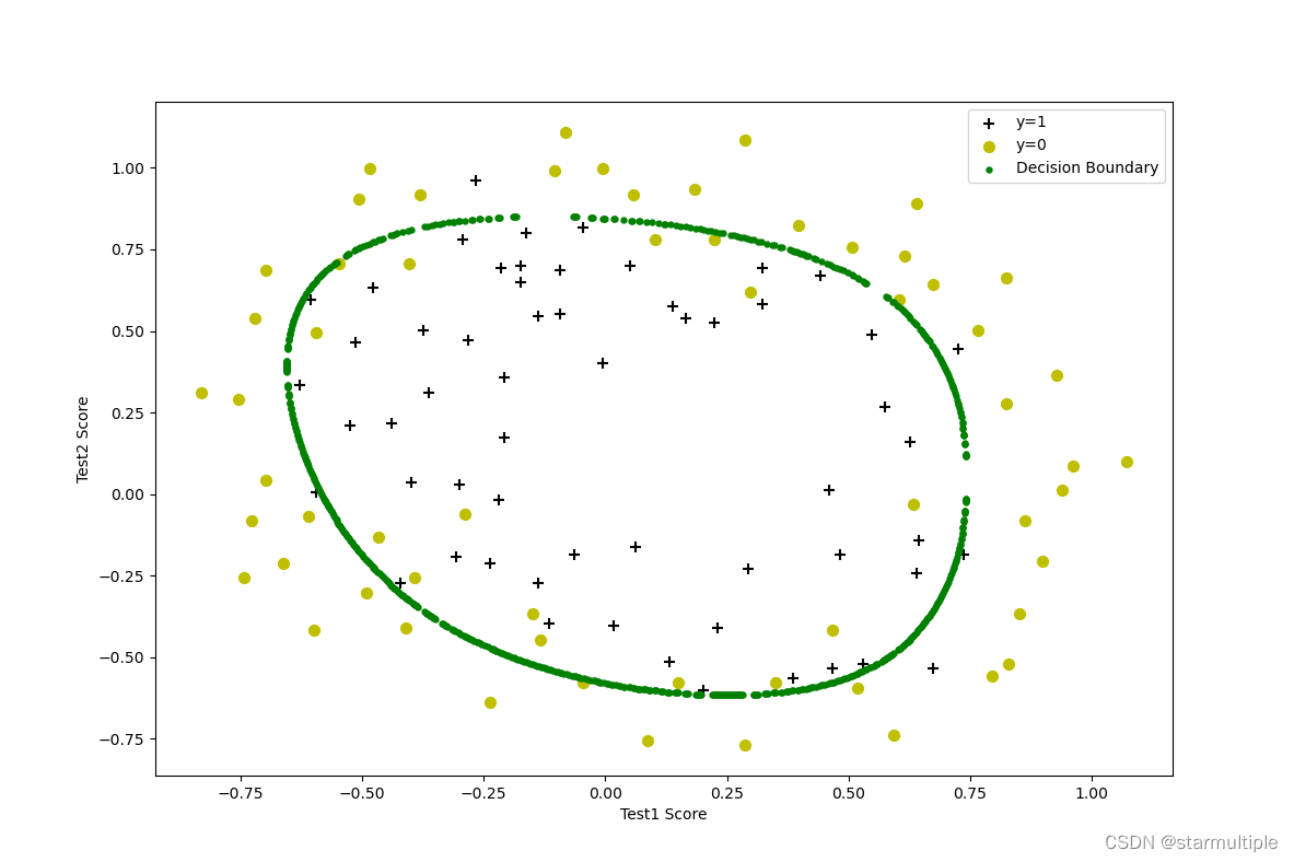
# 画决策边界
def draw_boundary(power, l):
    density = 1000
    threshhold = 2 * 10 ** -3

    theta = find_theta(power, l)
    x, y = find_decision_boundary(density, power, theta, threshhold)
    pos = df[df['Accepted'].isin([1])]
    neg = df[df['Accepted'].isin([0])]

    fig, ax = plt.subplots(figsize=(12, 8))
    ax.scatter(pos['Test1'], pos['Test2'], s=50, c='black', marker='+', label='y=1')
    ax.scatter(neg['Test1'], neg['Test2'], s=50, c='y', marker='o', label='y=0')
    ax.scatter(x, y, s=50, c='g', marker='.', label='Decision Boundary')
    ax.legend()
    ax.set_xlabel('Test1 Score')
    ax.set_ylabel('Test2 Score')

    plt.show()
draw_boundary(6, l=1)