当前位置:网站首页>hands-on-data-analysis 第三单元 模型搭建和评估
hands-on-data-analysis 第三单元 模型搭建和评估
2022-06-26 13:08:00 【沧夜2021】
hands-on-data-analysis 第三单元 模型搭建和评估
文章目录
1.模型搭建
1.1.导入相关库
import pandas as pd
import numpy as np
# matplotlib.pyplot 和 seaborn 是绘图库
import matplotlib.pyplot as plt
import seaborn as sns
from IPython.display import Image
# 内嵌显示图片
%matplotlib inline
plt.rcParams['font.sans-serif'] = ['SimHei']  # 用来正常显示中文标签
plt.rcParams['axes.unicode_minus'] = False  # 用来正常显示负号
plt.rcParams['figure.figsize'] = (10, 6)  # 设置输出图片大小
1.2.数据集的载入
# 读取原数据数集
train = pd.read_csv('train.csv')
train.shape
输出为:
(891, 12)
1.3.数据集分析
train.head()
输出为:
| PassengerId | Survived | Pclass | Name | Sex | Age | SibSp | Parch | Ticket | Fare | Cabin | Embarked | |
|---|---|---|---|---|---|---|---|---|---|---|---|---|
| 0 | 1 | 0 | 3 | Braund, Mr. Owen Harris | male | 22.0 | 1 | 0 | A/5 21171 | 7.2500 | NaN | S |
| 1 | 2 | 1 | 1 | Cumings, Mrs. John Bradley (Florence Briggs Th… | female | 38.0 | 1 | 0 | PC 17599 | 71.2833 | C85 | C |
| 2 | 3 | 1 | 3 | Heikkinen, Miss. Laina | female | 26.0 | 0 | 0 | STON/O2. 3101282 | 7.9250 | NaN | S |
| 3 | 4 | 1 | 1 | Futrelle, Mrs. Jacques Heath (Lily May Peel) | female | 35.0 | 1 | 0 | 113803 | 53.1000 | C123 | S |
| 4 | 5 | 0 | 3 | Allen, Mr. William Henry | male | 35.0 | 0 | 0 | 373450 | 8.0500 | NaN | S |
train.info()
<class 'pandas.core.frame.DataFrame'>
RangeIndex: 891 entries, 0 to 890
Data columns (total 12 columns):
 # Column Non-Null Count Dtype
---  ------       --------------  -----
 0   PassengerId  891 non-null    int64
 1   Survived     891 non-null    int64
 2   Pclass       891 non-null    int64
 3   Name         891 non-null    object
 4   Sex          891 non-null    object
 5   Age          714 non-null    float64
 6   SibSp        891 non-null    int64
 7   Parch        891 non-null    int64
 8   Ticket       891 non-null    object
 9   Fare         891 non-null    float64
 10  Cabin        204 non-null    object
 11  Embarked     889 non-null    object
dtypes: float64(2), int64(5), object(5)
memory usage: 83.7+ KB
可以看到这些数据还是需要清洗的,清洗过后的数据集如下:
#读取清洗过的数据集
data = pd.read_csv('clear_data.csv')
data.head()
| PassengerId | Pclass | Age | SibSp | Parch | Fare | Sex_female | Sex_male | Embarked_C | Embarked_Q | Embarked_S | |
|---|---|---|---|---|---|---|---|---|---|---|---|
| 0 | 0 | 3 | 22.0 | 1 | 0 | 7.2500 | 0 | 1 | 0 | 0 | 1 |
| 1 | 1 | 1 | 38.0 | 1 | 0 | 71.2833 | 1 | 0 | 1 | 0 | 0 |
| 2 | 2 | 3 | 26.0 | 0 | 0 | 7.9250 | 1 | 0 | 0 | 0 | 1 |
| 3 | 3 | 1 | 35.0 | 1 | 0 | 53.1000 | 1 | 0 | 0 | 0 | 1 |
| 4 | 4 | 3 | 35.0 | 0 | 0 | 8.0500 | 0 | 1 | 0 | 0 | 1 |
data.info()
输出为:
<class 'pandas.core.frame.DataFrame'>
RangeIndex: 891 entries, 0 to 890
Data columns (total 11 columns):
 # Column Non-Null Count Dtype
---  ------       --------------  -----
 0   PassengerId  891 non-null    int64
 1   Pclass       891 non-null    int64
 2   Age          891 non-null    float64
 3   SibSp        891 non-null    int64
 4   Parch        891 non-null    int64
 5   Fare         891 non-null    float64
 6   Sex_female   891 non-null    int64
 7   Sex_male     891 non-null    int64
 8   Embarked_C   891 non-null    int64
 9   Embarked_Q   891 non-null    int64
 10  Embarked_S   891 non-null    int64
dtypes: float64(2), int64(9)
memory usage: 76.7 KB
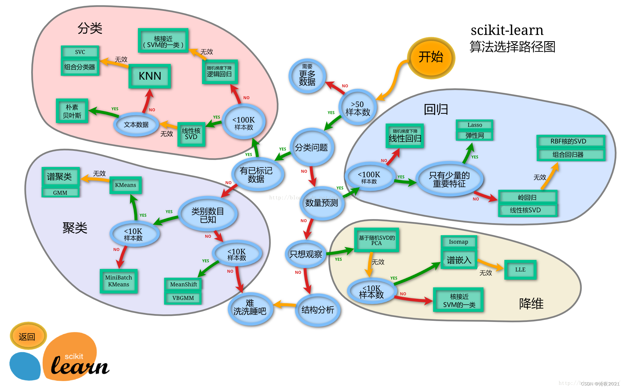
1.4.模型搭建
sklearn的算法选择路径
分割数据集
# train_test_split 是用来切割数据集的函数
from sklearn.model_selection import train_test_split
# 一般先取出X和y后再切割,有些情况会使用到未切割的,这时候X和y就可以用,x是清洗好的数据,y是我们要预测的存活数据'Survived'
X = data
y = train['Survived']
# 对数据集进行切割
X_train, X_test, y_train, y_test = train_test_split(X, y, stratify=y, random_state=0)
# 查看数据形状
X_train.shape, X_test.shape
输出为:
((668, 11), (223, 11))
X_train.info()
输出为:
<class 'pandas.core.frame.DataFrame'>
Int64Index: 668 entries, 671 to 80
Data columns (total 11 columns):
 # Column Non-Null Count Dtype
---  ------       --------------  -----
 0   PassengerId  668 non-null    int64
 1   Pclass       668 non-null    int64
 2   Age          668 non-null    float64
 3   SibSp        668 non-null    int64
 4   Parch        668 non-null    int64
 5   Fare         668 non-null    float64
 6   Sex_female   668 non-null    int64
 7   Sex_male     668 non-null    int64
 8   Embarked_C   668 non-null    int64
 9   Embarked_Q   668 non-null    int64
 10  Embarked_S   668 non-null    int64
dtypes: float64(2), int64(9)
memory usage: 82.6 KB
X_test.info()
输出为:
<class 'pandas.core.frame.DataFrame'>
Int64Index: 223 entries, 288 to 633
Data columns (total 11 columns):
 # Column Non-Null Count Dtype
---  ------       --------------  -----
 0   PassengerId  223 non-null    int64
 1   Pclass       223 non-null    int64
 2   Age          223 non-null    float64
 3   SibSp        223 non-null    int64
 4   Parch        223 non-null    int64
 5   Fare         223 non-null    float64
 6   Sex_female   223 non-null    int64
 7   Sex_male     223 non-null    int64
 8   Embarked_C   223 non-null    int64
 9   Embarked_Q   223 non-null    int64
 10  Embarked_S   223 non-null    int64
dtypes: float64(2), int64(9)
memory usage: 30.9 KB
1.5.导入模型
1.5.1.默认参数的逻辑回归模型
from sklearn.linear_model import LogisticRegression
from sklearn.ensemble import RandomForestClassifier
lr = LogisticRegression()
lr.fit(X_train, y_train)
输出为:
LogisticRegression(C=1.0, class_weight=None, dual=False, fit_intercept=True,
                   intercept_scaling=1, l1_ratio=None, max_iter=100,
                   multi_class='auto', n_jobs=None, penalty='l2',
                   random_state=None, solver='lbfgs', tol=0.0001, verbose=0,
                   warm_start=False)
# 查看训练集和测试集score值
print("Training set score: {:.2f}".format(lr.score(X_train, y_train)))
print("Testing set score: {:.2f}".format(lr.score(X_test, y_test)))
Training set score: 0.80
Testing set score: 0.79
1.5.2.调节参数的逻辑回归模型
lr2 = LogisticRegression(C=100)
lr2.fit(X_train, y_train)
输出为:
LogisticRegression(C=100, class_weight=None, dual=False, fit_intercept=True,
                   intercept_scaling=1, l1_ratio=None, max_iter=100,
                   multi_class='auto', n_jobs=None, penalty='l2',
                   random_state=None, solver='lbfgs', tol=0.0001, verbose=0,
                   warm_start=False)
print("Training set score: {:.2f}".format(lr2.score(X_train, y_train)))
print("Testing set score: {:.2f}".format(lr2.score(X_test, y_test)))
输出为:
Training set score: 0.79
Testing set score: 0.78
1.5.3.默认参数的随机森林分类模型
rfc = RandomForestClassifier()
rfc.fit(X_train, y_train)
输出为:
RandomForestClassifier(bootstrap=True, ccp_alpha=0.0, class_weight=None,
                       criterion='gini', max_depth=None, max_features='auto',
                       max_leaf_nodes=None, max_samples=None,
                       min_impurity_decrease=0.0, min_impurity_split=None,
                       min_samples_leaf=1, min_samples_split=2,
                       min_weight_fraction_leaf=0.0, n_estimators=100,
                       n_jobs=None, oob_score=False, random_state=None,
                       verbose=0, warm_start=False)
print("Training set score: {:.2f}".format(rfc.score(X_train, y_train)))
print("Testing set score: {:.2f}".format(rfc.score(X_test, y_test)))
输出为:
Training set score: 1.00
Testing set score: 0.82
1.5.4.调整参数后的随机森林分类模型
rfc2 = RandomForestClassifier(n_estimators=100, max_depth=5)
rfc2.fit(X_train, y_train)
输出为:
RandomForestClassifier(bootstrap=True, ccp_alpha=0.0, class_weight=None,
                       criterion='gini', max_depth=5, max_features='auto',
                       max_leaf_nodes=None, max_samples=None,
                       min_impurity_decrease=0.0, min_impurity_split=None,
                       min_samples_leaf=1, min_samples_split=2,
                       min_weight_fraction_leaf=0.0, n_estimators=100,
                       n_jobs=None, oob_score=False, random_state=None,
                       verbose=0, warm_start=False)
print("Training set score: {:.2f}".format(rfc2.score(X_train, y_train)))
print("Testing set score: {:.2f}".format(rfc2.score(X_test, y_test)))
输出为:
Training set score: 0.87
Testing set score: 0.81
1.6.预测模型
一般监督模型在sklearn里面有个predict能输出预测标签,predict_proba则可以输出标签概率
# 预测标签
pred = lr.predict(X_train)
# 此时我们可以看到0和1的数组
pred[:10]
输出为:
array([0, 1, 1, 1, 0, 0, 1, 0, 1, 1])
# 预测标签概率
pred_proba = lr.predict_proba(X_train)
pred_proba[:10]
输出为:
array([[0.60884602, 0.39115398],
       [0.17563455, 0.82436545],
       [0.40454114, 0.59545886],
       [0.1884778 , 0.8115222 ],
       [0.88013064, 0.11986936],
       [0.91411123, 0.08588877],
       [0.13260197, 0.86739803],
       [0.90571178, 0.09428822],
       [0.05273217, 0.94726783],
       [0.10924951, 0.89075049]])
2.模型评估
2.1.交叉验证
交叉验证有很多种,第一种是最简单的,也是很容易就想到的:把数据集分成两部分,一个是训练集(training set),一个是测试集(test set)。
不过,这个简单的方法存在两个弊端。
1.最终模型与参数的选取将极大程度依赖于你对训练集和测试集的划分方法。
2.该方法只用了部分数据进行模型的训练,未能充分利用数据集的数据。
为了解决这个问题,后面的技术人员进行了多种优化,接下来提到的就是K折交叉验证:
我们每次的测试集将不再只包含一个数据,而是多个,具体数目将根据K的选取决定。比如,如果K=5,那么我们利用七折交叉验证的步骤就是:
1.将所有数据集分成7份
2.不重复地每次取其中一份做测试集,用其他 6 份做训练集训练模型,之后计算该模型在测试集上的MSE
3.将7次的取平均得到最后的MSE

from sklearn.model_selection import cross_val_score
lr = LogisticRegression(C=100)
scores = cross_val_score(lr, X_train, y_train, cv=10)
# k折交叉验证分数
scores
输出:
array([0.82089552, 0.74626866, 0.74626866, 0.7761194 , 0.88059701,
       0.8358209 , 0.76119403, 0.8358209 , 0.74242424, 0.75757576])
# 平均交叉验证分数
print("Average cross-validation score: {:.2f}".format(scores.mean()))
输出:
Average cross-validation score: 0.79
2.2.混淆矩阵
混淆矩阵是用来总结一个分类器结果的矩阵。对于k元分类,其实它就是一个k x k的表格,用来记录分类器的预测结果。

混淆矩阵的方法在sklearn中的sklearn.metrics模块
混淆矩阵需要输入真实标签和预测标签
精确率、召回率以及f-分数可使用classification_report模块
实际上模型的好坏,看混淆矩阵的主对角线即可。
from sklearn.metrics import confusion_matrix
# 训练模型
lr = LogisticRegression(C=100)
lr.fit(X_train, y_train)
LogisticRegression(C=100, class_weight=None, dual=False, fit_intercept=True,
                   intercept_scaling=1, l1_ratio=None, max_iter=100,
                   multi_class='auto', n_jobs=None, penalty='l2',
                   random_state=None, solver='lbfgs', tol=0.0001, verbose=0,
                   warm_start=False)
# 模型预测结果
pred = lr.predict(X_train)
# 混淆矩阵
confusion_matrix(y_train, pred)
array([[354,  58],
       [ 83, 173]])
# 分类报告
from sklearn.metrics import classification_report
# 精确率、召回率以及f1-score
print(classification_report(y_train, pred))
    			precision    recall  f1-score   support

           0       0.81      0.86      0.83       412
           1       0.75      0.68      0.71       256

    accuracy                           0.79       668
   macro avg       0.78      0.77      0.77       668
weighted avg       0.79      0.79      0.79       668
2.3.ROC曲线
ROC曲线起源于第二次世界大战时期雷达兵对雷达的信号判断。当时每一个雷达兵的任务就是去解析雷达的信号,但是当时的雷达技术还没有那么先进,存在很多噪声,所以每当有信号出现在雷达屏幕上,雷达兵就需要对其进行破译。有的雷达兵比较谨慎,凡是有信号过来,他都会倾向于解析成是敌军轰炸机,有的雷达兵又比较神经大条,会倾向于解析成是飞鸟。在这种情况下就急需一套评估指标来帮助他汇总每一个雷达兵的预测信息以及来评估这台雷达的可靠性。于是,最早的ROC曲线分析方法就诞生了。在那之后,ROC曲线就被广泛运用于医学以及机器学习领域。
ROC的全称是Receiver Operating Characteristic Curve,中文名字叫【受试者工作特征曲线】
ROC曲线在sklearn中的模块为sklearn.metrics
ROC曲线下面所包围的面积越大越好
from sklearn.metrics import roc_curve
fpr, tpr, thresholds = roc_curve(y_test, lr.decision_function(X_test))
plt.plot(fpr, tpr, label="ROC Curve")
plt.xlabel("FPR")
plt.ylabel("TPR (recall)")
# 找到最接近于0的阈值
close_zero = np.argmin(np.abs(thresholds))
plt.plot(fpr[close_zero], tpr[close_zero], 'o', markersize=10, label="threshold zero", fillstyle="none", c='k', mew=2)
plt.legend(loc=4)

3.参考资料
边栏推荐
- Select tag - uses the default text as a placeholder prompt but is not considered a valid value
- MySQL讲解(二)
- character constants
- Ring queue PHP
- A primary multithreaded server model
- MediaPipe手势(Hands)
- D中不用GC
- 2021-10-18 character array
- Solutions to insufficient display permissions of find and Du -sh
- Logical operation
猜你喜欢

Chapter 10 setting up structured logging (2)

MySQL数据库常见故障——遗忘数据库密码
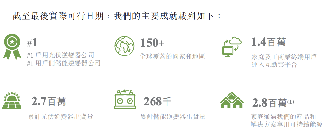
Guruiwat rushed to the Hong Kong stock exchange for listing: set "multiple firsts" and obtained an investment of 900million yuan from IDG capital

8.Ribbon负载均衡服务调用
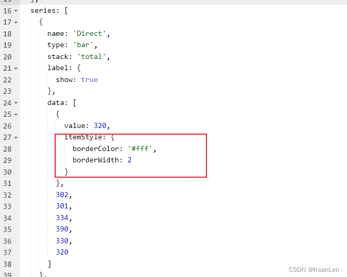
Echart stack histogram: add white spacing effect setting between color blocks
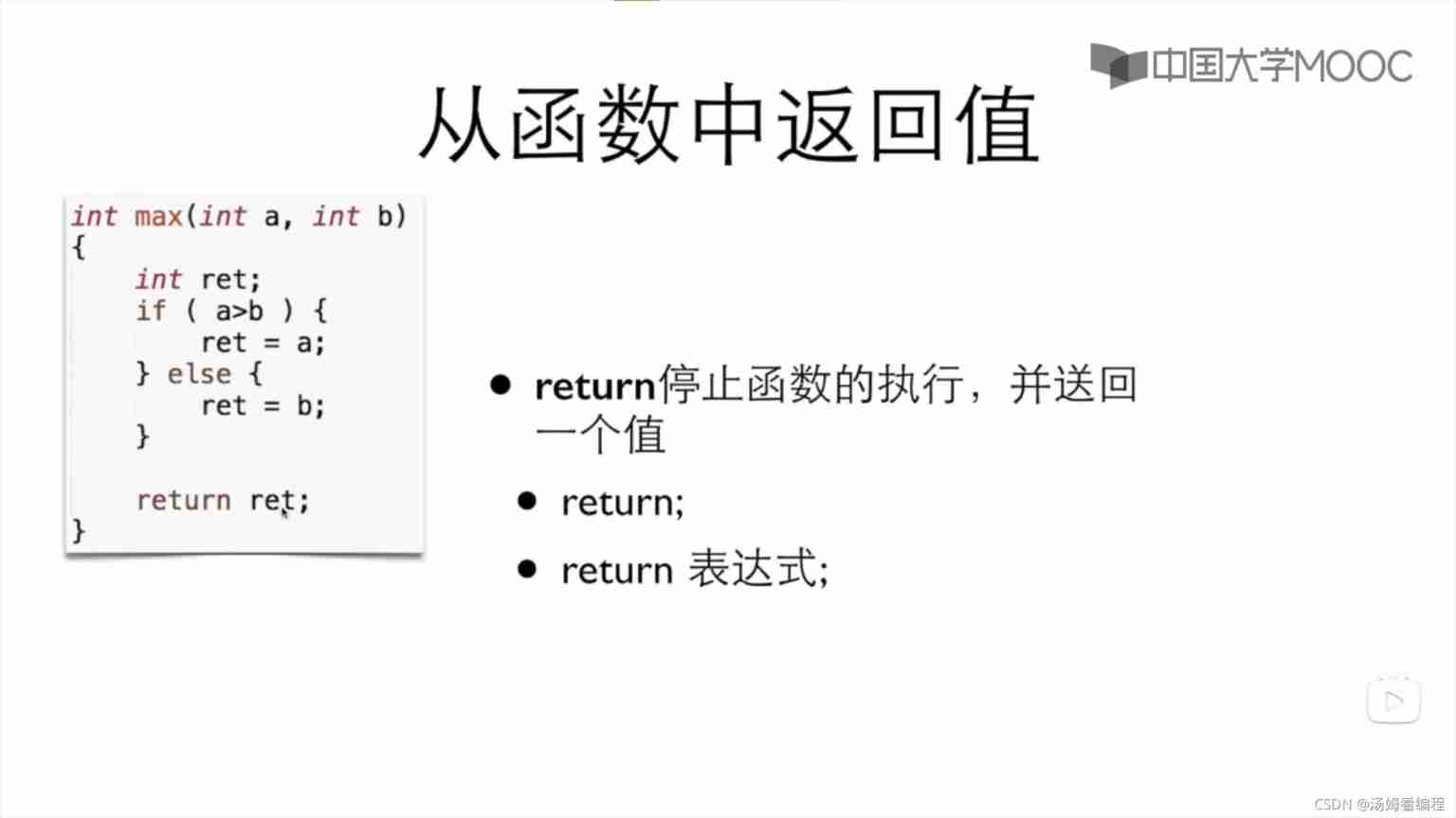
Zero basics of C language lesson 8: Functions

Create your own cross domain proxy server

HW蓝队溯源流程详细整理

微信小程序注册指引

Stack, LIFO
随机推荐
12 SQL optimization schemes summarized by old drivers (very practical)
MongoDB系列之适用场景和不适用场景
LAMP编译安装
[node.js] MySQL module
Es snapshot based data backup and restore
Guruiwat rushed to the Hong Kong stock exchange for listing: set "multiple firsts" and obtained an investment of 900million yuan from IDG capital
Mysql database explanation (6)
shell脚本详细介绍(四)
使用 Performance 看看浏览器在做什么
Traverse the specified directory to obtain the file name with the specified suffix (such as txt and INI) under the current directory
Applicable and inapplicable scenarios of mongodb series
Here Document免交互及Expect自动化交互
计算两点之间的距离(二维、三维)
7.Consul服务注册与发现
Jenkins build prompt error: eacces: permission denied
ES6 module
Echart stack histogram: add white spacing effect setting between color blocks
【MySQL从入门到精通】【高级篇】(二)MySQL目录结构与表在文件系统中的表示
Beifu PLC obtains system time, local time, current time zone and system time zone conversion through program
同花顺股票开户选哪个证券公司是比较好,比较安全的