当前位置:网站首页>Casadi -- detailed explanation of data types and introduction to basic operations
Casadi -- detailed explanation of data types and introduction to basic operations
2022-07-27 16:39:00 【An audience who doesn't understand music】
List of articles
1. Common symbols
1.1 SX Symbol
SX The data type is used to represent the matrix , Its elements are composed of symbolic expressions composed of a series of unary and binary operation sequences . To see how it works in practice , Please start interactive Python shell( for example , By getting from Linux Terminal or in integrated development environment ( Such as Spyder) Type in ipython) Or start MATLAB or Octave The graphical user interface . hypothesis CasADi Installed correctly , You can import the library into the workspace , As shown below :
from casadi import *
Create a variable using the following syntax x:
x = MX.sym("x")
print(x)
After running, the output is :
x
The above code creates a 1×1 matrix , That is, a name called x Symbolic primitives of ( It's a scalar ). This is just the display name , Instead of identifiers . Multiple variables can have the same name , But it's still different . The identifier is the return value . Besides , You can also call functions SX.sym ( With parameters ) To create vector or matrix valued symbolic variables :
y = SX.sym('y',5)
Z = SX.sym('Z',4,2)
print(y)
print(z)
After running, the output is :
[y_0, y_1, y_2, y_3, y_4]
[[Z_0, Z_4],
[Z_1, Z_5],
[Z_2, Z_6],
[Z_3, Z_7]]
The above code creates a 5×1 matrix ( The vector ) And a symbol primitive 4×2 matrix . SX.sym It's a ( static state ) function , It returns a SX example . After variable declaration , Now you can form expressions in an intuitive way :
f = x**2 + 10
f = sqrt(f)
print(f)
After running, the output is :
sqrt((10+sq(x)))
besides , You can also create a constant that does not exist SX example :
B1 = SX.zeros(4,5): #  An all zero dense  4×5  Empty matrix
B2 = SX(4,5): #  All zero sparse  4×5  Empty matrix
B4 = SX.eye(4): #  sparse 4×4 matrix , The diagonal to 1
print(B1)
print(B2)
print(B4)
After running, the output is :
B1: @1=0,
[[@1, @1, @1, @1, @1],
[@1, @1, @1, @1, @1],
[@1, @1, @1, @1, @1],
[@1, @1, @1, @1, @1]]
B2:
[[00, 00, 00, 00, 00],
[00, 00, 00, 00, 00],
[00, 00, 00, 00, 00],
[00, 00, 00, 00, 00]]
B4: @1=1,
[[@1, 00, 00, 00],
[00, @1, 00, 00],
[00, 00, @1, 00],
[00, 00, 00, @1]]
Be careful : Notice the difference between the above expressions : When printing with Structure zero ( Elements in a sparse matrix that are not explicitly assigned ) The expression of , These zeros will be expressed as 00, To connect them with Actual zero @1 ( Actually explicitly assigned elements ,print After use @1 To express 0, In order to distinguish between structural zero and actual zero ) Distinguish .
In addition to the above methods of use , The following table lists the commonly used SX expression :
| Function expression | purpose |
|---|---|
| SX.sym(name,n,m) | Create a n×m Symbolic primitives |
| SX.zeros(n,m) | Create a... With all elements zero n×m Dense matrix |
| SX(n,m) | Create a with zero elements n×m sparse matrix |
| SX.ones(n,m) | Create one that contains all 1 Of n×m Dense matrix |
| SX.eye(n) | Create a n×n Diagonal matrix , The diagonal element is 1, Elsewhere, the element structure is zero |
| SX(scalar_type) | Create a scalar using the value given by the parameter (1×1 matrix ), You can use this method explicitly , for example SX(9), Or implicit , for example 9 * SX.ones(2,2) |
| SX(matrix_type) | Create a matrix of a given numerical matrix , The numerical matrix is NumPy or SciPy matrix ( stay Python in ) Or dense or sparse matrix ( stay MATLAB / Octave in ). stay MATLAB/Octave in , for example SX([1,2,3,4]) Represents the row vector ,SX([1;2;3;4]) Represents the column vector ,SX([1,2;3,4]) Express 2×2 matrix , This method can be used explicitly or implicitly . |
| repmat(v,n,m) | Expression v Repeat the table vertically n Time , Repeat horizontally m Time . for example :repmat(SX(3),2,1) Create one with all elements as 3 Of 2×1 matrix . |
| SX(list) ( Limited to Python) | Create a column vector using the elements in the list (n×1 matrix ), for example SX([1,2,3,4]).( Be careful Python List and MATLAB/Octave The difference between horizontal series , Both use square bracket syntax ) |
| SX(list of list)( Limited to Python) | Use the elements in the list to create a dense matrix , for example SX([[1,2],[3,4]]) Or use SX([[1,2,3,4]]) Create a (1×n matrix ) Row vector . |
1.2 DM Symbol
DM And SX Very similar , But the difference is that non-zero elements are numeric rather than symbolic expressions . DM Syntax and SX Also the same , Except in part similar to SX.sym Such as function .
DM Mainly used in CasADi Store the matrix and the input and output as a function . It is not intended for compute intensive computing . So , Please use MATLAB Built in dense or sparse data types in 、Python Medium NumPy or SciPy Matrix or expression template based library , for example C++ Medium eigen、ublas or MTL. The conversion between types is usually simple :
C = DM(2,3)

C_dense = C.full()
from numpy import array
C_dense = array(C) # equivalent

C_sparse = C.sparse()
from scipy.sparse import csc_matrix
C_sparse = csc_matrix(C) # equivalent
SX More usage examples of can be found in http://install.casadi.org/ Found in the sample package . About such ( And other classes ) Documentation for specific functions , for example C++ API, Can be in http://docs.casadi.org/ Found on the .
1.3 MX Symbol
The output of the following code is a 2×2 matrix , Pay attention to the first sentence here @1=3, This means that in the output of the second line @1 representative 3, The output means CasADi For matrix f Each entry of creates a new expression (SX type ).
x = SX.sym('x',2,2)
y = SX.sym('y')
f = 3*x + y
print(f)
print(f.shape)
After running, the output is :
@1=3,
[[((@1x_0)+y), ((@1x_2)+y)],
[((@1x_1)+y), ((@1x_3)+y)]]
(2, 2)
In addition to the way above , We can also use a second, more general type of matrix expression MX. MX Types are allowed like SX Build an expression that consists of a series of basic operations . But with SX The difference is , These operations are not limited to scalar or binary basic operations ( R → R \mathbb{R}→\mathbb{R} R→R or R × R → R \mathbb{R}×\mathbb{R}→\mathbb{R} R×R→R). In its place , Used to form MX The basic operation of the expression can input multiple sparse matrix values in general , Multiple sparse matrix valued output functions : R n 1 × m 1 × … × R n N × m N → R p 1 × q 1 × … × R p M × q M \mathbb{R}^{ {n_1}×{m_1}}×…×\mathbb{R}^{ {n_N}×{m_N}}→\mathbb{R}^{ {p_1}×{q_1}}×…×\mathbb{R}^{ {p_M}×{q_M}} Rn1×m1×…×RnN×mN→Rp1×q1×…×RpM×qM, for example :
x = MX.sym('x',2,2)
y = MX.sym('y')
f = 3*x + y
print(f)
print(f.shape)
After running, the output is :
((3*x)+y)
(2, 2)
The results of the above two codes are the same , MX The symbol consists of only two operations ( A multiplication and an addition ) form , and SX There are eight equivalents ( Each element consists of two ,f(1,1) from (@1x_0) and y constitute ). therefore , When using operations with natural vector or matrix values with many elements ,MX Can be more economical .
MX Support the use of SX The same syntax to get and set elements , But the implementation is very different . for example , Test printing 2×2 The upper left corner of the symbolic element :
x = MX.sym('x',2,2)
print(x[0,0])
The output should be understood to be equal to x One of the first ( namely C++ Index in 0) Expression of non-zero elements in structure , With the above SX Cases of x_0 Different , It's the first ( Indexes 0) The position of the matrix .
When setting elements, the usage is similar :
x = MX.sym('x',2)
A = MX(2,2)
A[0,0] = x[0]
A[1,1] = x[0]+x[1]
print('A:', A)
After running, the output is :
A: (project((zeros(2x2,1nz)[0] = x[0]))[1] = (x[0]+x[1]))
This output can be understood as : Start with an all zero sparse matrix , An element is assigned to x_0. Then it is projected to matrices with different sparsity , And assign another element to x_0+x_1.
1.4 SX and MX Mixing
Can't be SX Object and the MX Multiply objects , Nor can you do anything else to mix the two in the same expression diagram . But it can be in MX The figure includes a pair of SX Call of the function defined by the expression . If you need to improve the efficiency of the program , It can be mixed SX and MX, Because the SX The cost of each operation of the function defined by the expression is much lower , This makes the system complete a series of scalar operations faster . therefore ,SX Expressions are intended for low-level operations , and MX Expressions are used to implement responsible operations , For example, implement NLP Constraint function of .
1.5 Sparse class
CasADi The matrix in uses compressed columns to store (CCS) Format for storage . This is the standard format for sparse matrices , Allows efficient execution of linear algebraic operations , For example, element by element operation 、 Matrix multiplication and transpose . stay CCS In the format , Sparse mode uses dimensions ( Number of rows and columns ) And two vectors to decode . The first vector contains the index of the first structurally non-zero element of each column , The second vector contains the row index of each non-zero element . of CCS More details on format , See for example Netlib Template for linear system solutions on . Please note that ,CasADi Use... For sparse and dense matrices CCS Format .
CasADi The sparse pattern in is stored as Sparsity Class , This class is reference counted , This means that multiple matrices can share the same sparse pattern , Include MX Expression graph and SX and DM Example . Sparse classes are also cached , This means that you always avoid creating multiple instances of the same sparse pattern .
The following list summarizes the most common methods of building new sparse patterns :
| Function name | function |
|---|---|
| Sparsity.dense(n,m) | Create a dense n×m Sparse mode |
| Sparsity(n,m) | Create a sparse n×m Sparse mode |
| Sparsity.diag(n) | Create diagonal lines n×n Sparse mode |
| Sparsity.upper(n) | Create an upper triangle n×n Sparse mode |
| Sparsity.lower(n) | Create a lower triangle n×n Sparse mode |
Sparse classes can be used to create nonstandard matrices , for example :
print(SX.sym('x',Sparsity.lower(3)))
After running, the output is :
[[x_0, 00, 00],
[x_1, x_3, 00],
[x_2, x_4, x_5]]
1.5.1 Gets and sets the elements in the matrix
To get or set CasADi Matrix type (SX、MX and DM) An element or group of elements in , We are Python Square brackets are used in , stay C++ and MATLAB Use parentheses in . According to the conventions of these languages , Index in C++ and Python In the from 0 Start , And in the MATLAB In the from 1 Start . stay Python and C++ in , We allow negative indexes to specify indexes that count from the end . stay MATLAB in , Use end Keywords start at the end of the index .
Indexing can be done with one or two indexes . Use two indexes , You can access specific lines ( Or one or more lines ) And specific columns ( Or a set of columns ). Use an index , You can access an element ( Or a set of elements ), From the top left corner , Press the column to the lower right corner . Whether structurally zero or not , All elements are counted . for example :
M = SX([[3,7],[4,5]])
print(M[0,:])
M[0,:] = 1
print(M)
After running, the output is :
[[3, 7]]
@1=1,
[[@1, @1],
[4, 5]]
And Python Of NumPy Different ,CasADi The fragment is not a view of the left data ; contrary , Fragment access (Slice access) Copy the data . therefore , In the following example , matrix m There's no change at all :
M = SX([[3,7],[4,5]])
M[0,:][0,0] = 1
print(M)
After running, the output is :
[[3, 7],
[4, 5]]
The following describes how to get and set matrix elements in detail . This discussion applies to CasADi All matrix types .
By providing row and column pairs or their flattening index ( Start from the upper left corner of the matrix, column by column ) To get or set single element access :
M = diag(SX([3,4,5,6]))
print(M)
After running, the output is :
[[3, 00, 00, 00],
[00, 4, 00, 00],
[00, 00, 5, 00],[00, 00, 00, 6]]
print(M[0,0])
print(M[1,0])
print(M[-1,-1])
After running, the output is :
3
00
6
Fragment access (Slice access) It means setting more than one element at a time . This is much more efficient than setting one element at a time . By providing (start , stop , step) Tuples to get or set fragments . stay Python and MATLAB in ,CasADi Use standard syntax :
print(M[:,1])
print(M[1:,1:4:2])  #  Corresponding (start , stop , step)
After running, the output is :
[00, 4, 00, 00]
[[4, 00],
[00, 00],
[00, 6]]
List access is similar to ( But the efficiency may be lower than ) Fragment access :
M = SX([[3,7,8,9],[4,5,6,1]])
print(M)
print(M[0,[0,3]], M[[5,-6]])
After running, the output is :
[[3, 7, 8, 9],
[4, 5, 6, 1]]
[[3, 9]] [6, 7]
1.6 Arithmetic operations
1.6.1 Multiplication
CasADi Supports most standard arithmetic operations , Such as addition 、 Multiplication 、 power 、 Trigonometric functions, etc :
x = SX.sym('x')
y = SX.sym('y',2,2)
print(sin(y)-x)
After running, the output is :
[[(sin(y_0)-x), (sin(y_2)-x)],
[(sin(y_1)-x), (sin(y_3)-x)]]
stay C++ and Python( But not in MATLAB in ) in , Standard multiplication ( Use *) Still used for element multiplication ( stay MATLAB .* in ). For matrix multiplication , Use A @ B or (mtimes(A,B) in Python 3.4+):
print(y*y, [email protected])
After running, the output is :
[[sq(y_0), sq(y_2)],
[sq(y_1), sq(y_3)]]
[[(sq(y_0)+(y_2*y_1)), ((y_0*y_2)+(y_2*y_3))],
[((y_1*y_0)+(y_3*y_1)), ((y_1*y_2)+sq(y_3))]]
according to MATLAB It's a convention in the world , When any parameter is scalar , Use * and .* The multiplication of is equivalent .
1.6.2 transpose
Transpose use Python Chinese grammar A.T、C++ Medium A.T() as well as A or A formation . stay MATLAB in :
print(y)
print(y.T)
After running, the output is :
[[y_0, y_2],
[y_1, y_3]][[y_0, y_1],
[y_2, y_3]]
1.6.3 reshape()
restore (reshape) It means changing the number of rows and columns , But keep the number of elements and the relative position of non-zero elements . This is a very low computational cost operation , It uses the following syntax to execute :
x = SX.eye(4)
print(reshape(x,2,8))
After running, the output is :
@1=1,
[[@1, 00, 00, 00, 00, @1, 00, 00],
[00, 00, @1, 00, 00, 00, 00, @1]]
1.6.4 vertcat()/horzcat()
Concatenation means stacking matrices horizontally or vertically . Because in CasADi The main way to store elements in columns , Horizontal stacking matrix is the most effective . It's actually a matrix of column vectors ( That is, it consists of a single column ) It can also be stacked vertically . Use Python and C++ The function in vertcat and horzcat( Use a variable number of input parameters ) And in MATLAB Use square brackets to perform vertical and horizontal connections in :
x = SX.sym('x',5)
y = SX.sym('y',5)
print(vertcat(x,y))
After running, the output is :
[x_0, x_1, x_2, x_3, x_4, y_0, y_1, y_2, y_3, y_4]
print(horzcat(x,y))
After running, the output is :
[[x_0, y_0],
[x_1, y_1],
[x_2, y_2],
[x_3, y_3],
[x_4, y_4]]
There are also some variations of these functions , They will list ( stay Python in ) An array or cell ( stay Matlab in ) As input :
L = [x,y]
print(hcat(L))
After running, the output is :
[[x_0, y_0],
[x_1, y_1],
[x_2, y_2],
[x_3, y_3],
[x_4, y_4]]
1.6.5 split
Horizontal and vertical splitting is the reverse operation of horizontal and vertical concatenation described above . To split the expression horizontally into n A smaller expression , In addition to the expression to be split , The length is also required n+1 Vector offset of . The first element of the offset vector must be 0, The last element must be the number of columns . The remaining elements must be arranged in non decreasing order . then , The output of the split operation i Include with o f f s e t [ i ] ≤ c < o f f s e t [ i + 1 ] offset[i]≤c<offset[i+1] offset[i]≤c<offset[i+1] The column of c. The following demonstrates the syntax :
x = SX.sym('x',5,2)
w = horzsplit(x,[0,1,2])
print(w[0], w[1])
After running, the output is :
[x_0, x_1, x_2, x_3, x_4] [x_5, x_6, x_7, x_8, x_9]
vertsplit The principle of operation is similar , But the offset vector refers to the row :
w = vertsplit(x,[0,3,5])
print(w[0], w[1])
After running, the output is :
[[x_0, x_5],
[x_1, x_6],
[x_2, x_7]]
[[x_3, x_8],
[x_4, x_9]]
For the above vertical split , Fragment access can be used instead of horizontal and vertical splitting :
w = [x[0:3,:], x[3:5,:]]
print(w[0], w[1])
After running, the output is :
[[x_0, x_5],
[x_1, x_6],
[x_2, x_7]]
[[x_3, x_8],
[x_4, x_9]]
about SX Variables created , This alternative method is completely equivalent , But for the MX chart , When all split expressions are needed , Use horzsplit/vertsplit It's much more efficient .
1.6.6 Inner product
Inner product , Defined as < A , B > : = t r ( A B ) = ∑ i , j A i , j B i , j <A,B>:=tr(AB)=∑_{i,j}A_{i,j}B_{i,j} <A,B>:=tr(AB)=∑i,jAi,jBi,j, Create as follows :
x = SX.sym('x',2,2)
print(dot(x,x))
After running, the output is :
(((sq(x_0)+sq(x_1))+sq(x_2))+sq(x_3))
Many of the above operations are also defined for sparse classes , after vertcat、horzsplit、 Transposition 、 Add ( Returns the union of two sparse patterns ) Sum and multiplication ( Returns the intersection of two sparse patterns ) The matrix returned after the operation is also sparse .
1.7 Query attribute
You can check whether the matrix or sparse pattern has specific properties by calling the appropriate member function . For example, query matrix size :
y = SX.sym('y',10,1)
print(y.shape)
After running, the output is :
(10, 1)
Query a matrix A The common operations of the properties of are as follows :
| Function name | function |
|---|---|
| A.size1() | Row number |
| A.size2() | Number of columns |
| A.shape | ( stay MATLAB Medium “size”) shape , to (nrow,ncol) |
| A.numel() | Element number , namely nrow∗ncol |
| A.nnz() | The number of structurally nonzero elements , If dense , It is equal to A.numel(). |
| A.sparsity() | Retrieve references to sparse patterns |
| A.is_dense() | Is a dense matrix , That is, there is no structure zero |
| A.is_scalar() | Whether the matrix is scalar , The dimension is 1×1? |
| A.is_column() | A matrix is a vector , The dimension is n Than 1? |
| A.is_square() | Is a matrix a square matrix ? |
| A.is_triu() | Is it a triangle on a matrix ? |
| A.is_constant() | Are all matrix terms constants ? |
| A.is_integer() | Are all matrix terms integer values ? |
1.8 linear algebra
CasADi Support a limited number of linear algebraic operations , for example For the solution of linear equations :
A = MX.sym('A',3,3)
b = MX.sym('b',3)
print(solve(A,b))
After running, the output is :
(A\b)
1.9 Differential and integral calculus - Algorithm differentiation
CasADi The core function is algorithmic(or automatic) differential (AD). For the function f : R N → R M f:\mathbb{R}^N→\mathbb{R}^M f:RN→RM:
y = f ( x ) , y=f(x), y=f(x),
Forward mode directional derivative (forward mode directional derivatives) Can be used to calculate Jacobian-times-vector The product of :
y ^ = ∂ f ∂ x x ^ \hat{y} = \frac{\partial f}{\partial x} \hat{x} y^=∂x∂fx^
Similarly , Directional derivative of reverse mode (reverse mode directional derivatives) It can be used to calculate the product of Jacobian transpose time vector :
x ^ = ( ∂ f ∂ x ) T y ^ \hat{x} = (\frac{\partial f}{\partial x})^T \hat{y} x^=(∂x∂f)Ty^
Calculation cost and evaluation of directional derivatives of forward and reverse modes f(x) In direct proportion to , And with the x Independent of the dimension of .
CasADi It can also effectively generate complete 、 Sparse Jacobian determinant . Its algorithm is very complex , But it basically includes the following steps :
- Automatic detection Jacobian Sparse mode of
- Use the graph coloring technique to find some forward and... Needed to build a complete Jacobian determinant / Or directional derivative
- Calculate the directional derivative numerically or symbolically
- Calculate the Jacobian determinant
Hessian The calculation method is to calculate the gradient first , Then perform the same steps as above , Calculate the Jacobian matrix of the gradient in the same way as above , At the same time, using symmetry .
1.9.1 syntax
Expression for calculating Jacobian determinant :
A = SX.sym('A',3,2)
x = SX.sym('x',2)
print(jacobian([email protected],x))
After running, the output is :
[[A_0, A_3],
[A_1, A_4],
[A_2, A_5]]
When the differential expression is scalar , You can also calculate the gradient in the sense of matrix :
print(gradient(dot(A,A),A))
After running, the output is :
[[(A_0+A_0), (A_3+A_3)],
[(A_1+A_1), (A_4+A_4)],
[(A_2+A_2), (A_5+A_5)]]
Please note that , And jacobian Different , The gradient always returns a dense vector .
Hessians And the gradient as a by-product is calculated as follows :
[H,g] = hessian(dot(x,x),x)
print('H:', H)
After running, the output is :
H: @1=2,
[[@1, 00],
[00, @1]]
For calculating the Jacobian multiplication vector product ,jtimes function —— Execute forward mode AD—— It is usually more effective than creating a complete Jacobian matrix and performing matrix vector multiplication :
A = DM([[1,3],[4,7],[2,8]])
x = SX.sym('x',2)
v = SX.sym('v',2)
f = mtimes(A,x)
print(jtimes(f,x,v))
After running, the output is :
[(v_0+(3v_1)), ((4v_0)+(7v_1)), ((2v_0)+(8*v_1))]
jtimes The function optionally computes the transposed Jacobian vector product , Reverse mode AD:
w = SX.sym('w',3)
f = mtimes(A,x)
print(jtimes(f,x,w,True))
After running, the output is :
[(((2w_2)+(4w_1))+w_0), (((8w_2)+(7w_1))+(3*w_0))]
边栏推荐
- Reduce PDF document size (Reprint)
- Sudden! 28 Chinese entities including Hikvision / Dahua / Shangtang / Kuangshi / ITU / iFLYTEK have been blacklisted by the United States
- Install MySQL using CentOS yum
- Embedded interview
- Json数据的格式使用
- 从零开始Blazor Server(1)--项目搭建
- Rotate the whole model in ADAMS
- 大数相加
- Coturn service installation in webrtc
- gpt-2 文本生成
猜你喜欢

ADAMS中转动整个模型
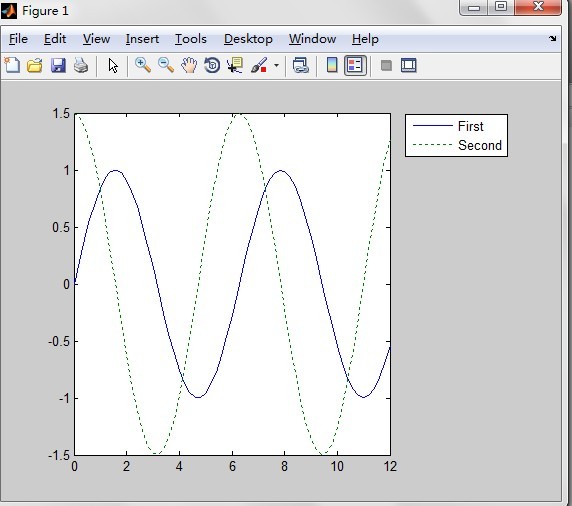
Matlab legend usage

The difference and use between get request and post request

Leetcode25 question: turn the linked list in a group of K -- detailed explanation of the difficult questions of the linked list

Supplement - example of integer programming

DRF learning notes (V): viewset
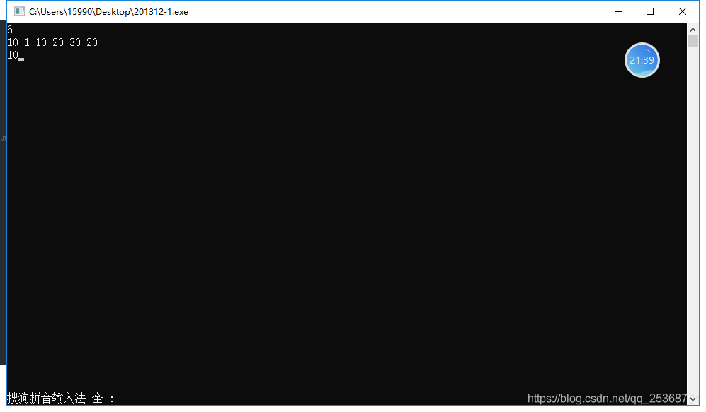
CCF-201312-1
![[paper reading] single- and cross modality near duplicate image pairsdetection via spatial transformer compare](/img/33/8af12d58f4afeb807ebf9a90a2ea47.png)
[paper reading] single- and cross modality near duplicate image pairsdetection via spatial transformer compare

Boolean value

Mazak handwheel maintenance Mazak little giant CNC machine tool handle operator maintenance av-eahs-382-1
随机推荐
Scala for loop (loop guard, loop step size, loop nesting, introducing variables, loop return value, loop interrupt breaks)
The solution to the memory exhaustion problem when PHP circulates a large amount of data
TP5 -- query field contains a certain --find of search criteria_ IN_ SET
Kmeans implementation
Two methods of generating excel table with PHP
The first week of C language learning - the history of C language
插入word中的图片保持高dpi方法
[paper reading] a CNN transformer hybrid approach for cropclassification using multitemporalmultisensor images
Opencv (II) -- basic image processing
获取当前时间的前N天和前后天的数组列表循环遍历每一天
COMS Technology
重新配置cubemx后,生成的代码用IAR打开不成功
Reduce PDF document size (Reprint)
Implementation of filler creator material editing tool
OpenCV(五)——运动目标识别
Sudden! 28 Chinese entities including Hikvision / Dahua / Shangtang / Kuangshi / ITU / iFLYTEK have been blacklisted by the United States
OpenCV(一)——图像基础知识
TP5 query empty two cases
Gpt-2 text generation
最大子段和 Go 四种的四种求解