当前位置:网站首页>深度学习Course2第二周Optimization Algorithms习题整理
深度学习Course2第二周Optimization Algorithms习题整理
2022-08-01 21:59:00 【l8947943】
Optimization Algorithms
- Using the notation for mini-batch gradient descent. To what of the following does a [ 2 ] { 4 } ( 3 ) a^{[2]\lbrace 4 \rbrace(3)} a[2]{ 4}(3) correspond?
- The activation of the third layer when the input is the fourth example of the second mini-batch.
- The activation of the second layer when the input is the third example of the fourth mini-batch.
- The activation of the fourth layer when the input is the second example of the third mini-batch.
- The activation of the second layer when the input is the fourth example of the third mini-batch.
- Which of these statements about mini-batch gradient descent do you agree with?
- You should implement mini-batch gradient descent without an explicit for-loop over different mini-batches so that the algorithm processes all mini-batches at the same time (vectorization).
- Training one epoch (one pass through the training set) using mini-batch gradient descent is faster than training one epoch using batch gradient descent.
- When the mini-batch size is the same as the training size, mini-batch gradient descent is equivalent to batch gradient descent.
(解释: Batch gradient descent uses all the examples at each iteration, this is equivalent to having only one mini-batch of the size of the complete training set in mini-batch gradient descent.)
- Why is the best mini-batch size usually not 1 and not m, but instead something in-between? Check all that are true.
- If the mini-batch size is 1, you lose the benefits of vectorization across examples in the mini-batch.
- If the mini-batch size is m, you end up with stochastic gradient descent, which is usually slower than mini-batch gradient descent.
- If the mini-batch size is 1, you end up having to process the entire training set before making any progress.
- If the mini-batch size is m, you end up with batch gradient descent, which has to process the whole training set before making progress.
- While using mini-batch gradient descent with a batch size larger than 1 but less than m, the plot of the cost function JJ looks like this:

You notice that the value of J J J is not always decreasing. Which of the following is the most likely reason for that?
- In mini-batch gradient descent we calculate J ( y ^ { t } , y { t } ) ) J(\hat{y} ^{\{t\}} ,{y} ^{\{t\}} )) J(y^{ t},y{ t})) thus with each batch we compute over a new set of data.
- A bad implementation of the backpropagation process, we should use gradient check to debug our implementation.
- You are not implementing the moving averages correctly. Using moving averages will smooth the graph.
- The algorithm is on a local minimum thus the noisy behavior.
(解释:Yes. Since at each iteration we work with a different set of data or batch the loss function doesn’t have to be decreasing at each iteration.)
- Suppose the temperature in Casablanca over the first two days of January are the same:
Jan 1st: θ 1 = 1 0 o C \theta_1 = 10^o C θ1=10oC
Jan 2nd: θ 2 = 1 0 o C \theta_2 = 10^oC θ2=10oC
(We used Fahrenheit in the lecture, so we will use Celsius here in honor of the metric world.)
Say you use an exponentially weighted average with β = 0.5 \beta = 0.5 β=0.5 to track the temperature: v 0 = 0 v_0 = 0 v0=0, v t = β v t − 1 + ( 1 − β ) θ t v_t = \beta v_{t-1} +(1-\beta)\theta_t vt=βvt−1+(1−β)θt. If v 2 v_2 v2 is the value computed after day 2 without bias correction, and v 2 c o r r e c t e d v_2^{corrected} v2corrected is the value you compute with bias correction. What are these values? (You might be able to do this without a calculator, but you don’t actually need one. Remember what bias correction is doing.)
- v 2 = 10 v_2=10 v2=10, v 2 c o r r e c t e d = 10 v^{corrected}_{2}=10 v2corrected=10
- v 2 = 7.5 v_2=7.5 v2=7.5, v 2 c o r r e c t e d = 7.5 v^{corrected}_{2}=7.5 v2corrected=7.5
- v 2 = 7.5 v_2=7.5 v2=7.5, v 2 c o r r e c t e d = 10 v^{corrected}_{2}=10 v2corrected=10
- v 2 = 10 v_2=10 v2=10, v 2 c o r r e c t e d = 7.5 v^{corrected}_{2}=7.5 v2corrected=7.5
- Which of the following is true about learning rate decay?
- The intuition behind it is that for later epochs our parameters are closer to a minimum thus it is more convenient to take smaller steps to prevent large oscillations.
- We use it to increase the size of the steps taken in each mini-batch iteration.
- The intuition behind it is that for later epochs our parameters are closer to a minimum thus it is more convenient to take larger steps to accelerate the convergence.
- It helps to reduce the variance of a model.
(解释:Reducing the learning rate with time reduces the oscillation around a minimum.)
- You use an exponentially weighted average on the London temperature dataset. You use the following to track the temperature: v t = β v t − 1 + ( 1 − β ) θ t v_{t} = \beta v_{t-1} + (1-\beta)\theta_t vt=βvt−1+(1−β)θt. The yellow and red lines were computed using values b e t a 1 beta_1 beta1 and b e t a 2 beta_2 beta2 respectively. Which of the following are true?
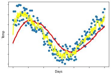
- β 1 < β 2 \beta_1<\beta_2 β1<β2
- β 1 = β 2 \beta_1=\beta_2 β1=β2
- β 1 > β 2 \beta_1>\beta_2 β1>β2
- β 1 = 0 , β 2 > 0 \beta_1=0,\beta_2>0 β1=0,β2>0
(解释:越向右越平滑,β越大)
- Consider the figure:

Suppose this plot was generated with gradient descent with momentum β = 0.01 \beta = 0.01 β=0.01. What happens if we increase the value of β \beta β to 0.1?
- The gradient descent process starts oscillating in the vertical direction.
- The gradient descent process starts moving more in the horizontal direction and less in the vertical.
- The gradient descent process moves less in the horizontal direction and more in the vertical direction.
- The gradient descent process moves more in the horizontal and the vertical axis.
(解释:随着β增大,走的步伐跨度越大,振幅越小,The use of a greater value of β causes a more efficient process thus reducing the oscillation in the horizontal direction and moving the steps more in the vertical direction.)
- Suppose batch gradient descent in a deep network is taking excessively long to find a value of the parameters that achieves a small value for the cost function J ( W [ 1 ] , b [ 1 ] , . . . , W [ L ] , b [ L ] ) \mathcal{J}(W^{[1]},b^{[1]},...,W^{[L]},b^{[L]}) J(W[1],b[1],...,W[L],b[L]). Which of the following techniques could help find parameter values that attain a small value for J \mathcal{J} J? (Check all that apply)
- Normalize the input data.
(解释:Yes. In some cases, if the scale of the features is very different, normalizing the input data will speed up the training process.) - Try better random initialization for the weights
(解释:Yes. As seen in previous lectures this can help the gradient descent process to prevent vanishing gradients.) - Add more data to the training set.
- Try using gradient descent with momentum.
(解释:Yes. The use of momentum can improve the speed of the training. Although other methods might give better results, such as Adam.)
- Which of the following are true about Adam?
- Adam can only be used with batch gradient descent and not with mini-batch gradient descent.
- The most important hyperparameter on Adam is ϵ ϵ ϵ and should be carefully tuned.
- Adam combines the advantages of RMSProp and momentum.
- Adam automatically tunes the hyperparameter α α α .
(解释:Precisely Adam combines the features of RMSProp and momentum that is why we use two-parameter β 1 β1 β1 and β 2 β2 β2, besides ϵ ϵ ϵ.)
边栏推荐
- shell programming conventions and variables
- Analysis of the development trend of game metaverse
- Advanced Algebra_Proof_The algebraic multiplicity of any eigenvalue of a matrix is greater than or equal to its geometric multiplicity
- 基于 OData 模型和 JSON 模型的 SAP UI5 表格控件行项目的添加和删除实现
- Lecture 3: Several common table field data types in MySQL database
- Uses of Anacoda
- long investment career
- ModuleNotFoundError: No module named 'yaml'
- SOM Network 2: Implementation of the Code
- 【C语言实现】求两个整数的较大值
猜你喜欢
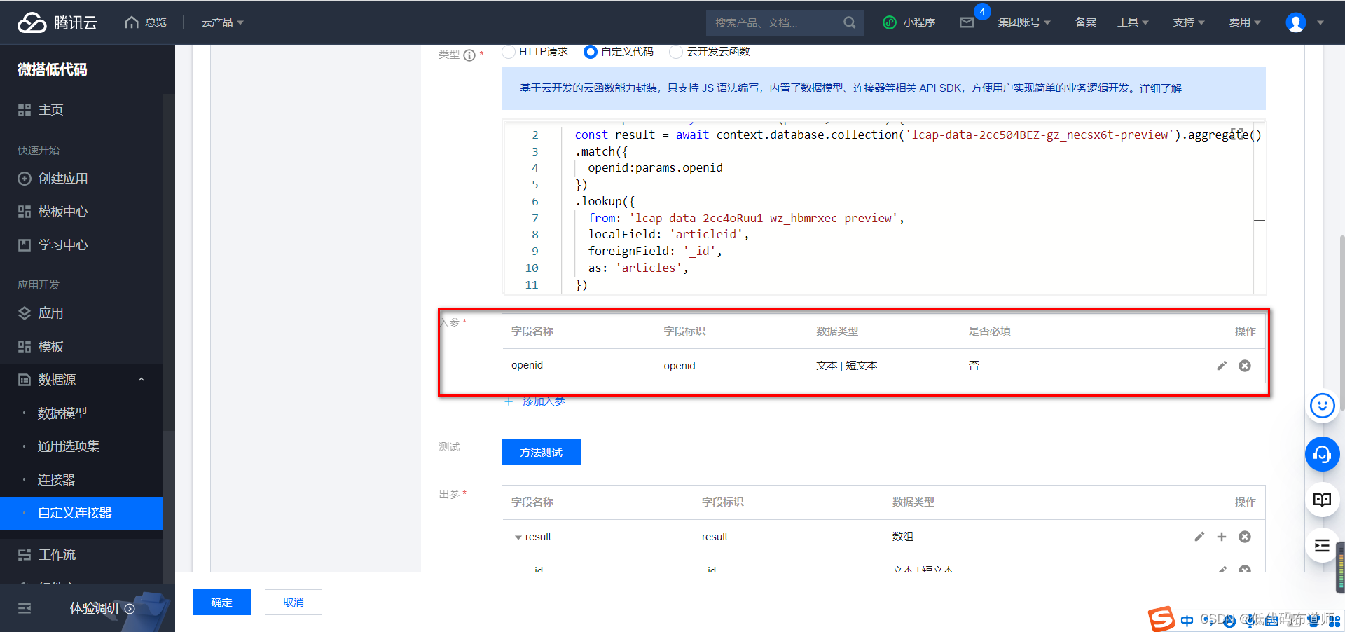
小程序中的多表联合查询

模拟数据之mockjs

Based on php hotel online reservation management system acquisition (php graduation project)
LeetCode952三部曲之二:小幅度优化(137ms -> 122ms,超39% -> 超51%)
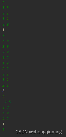
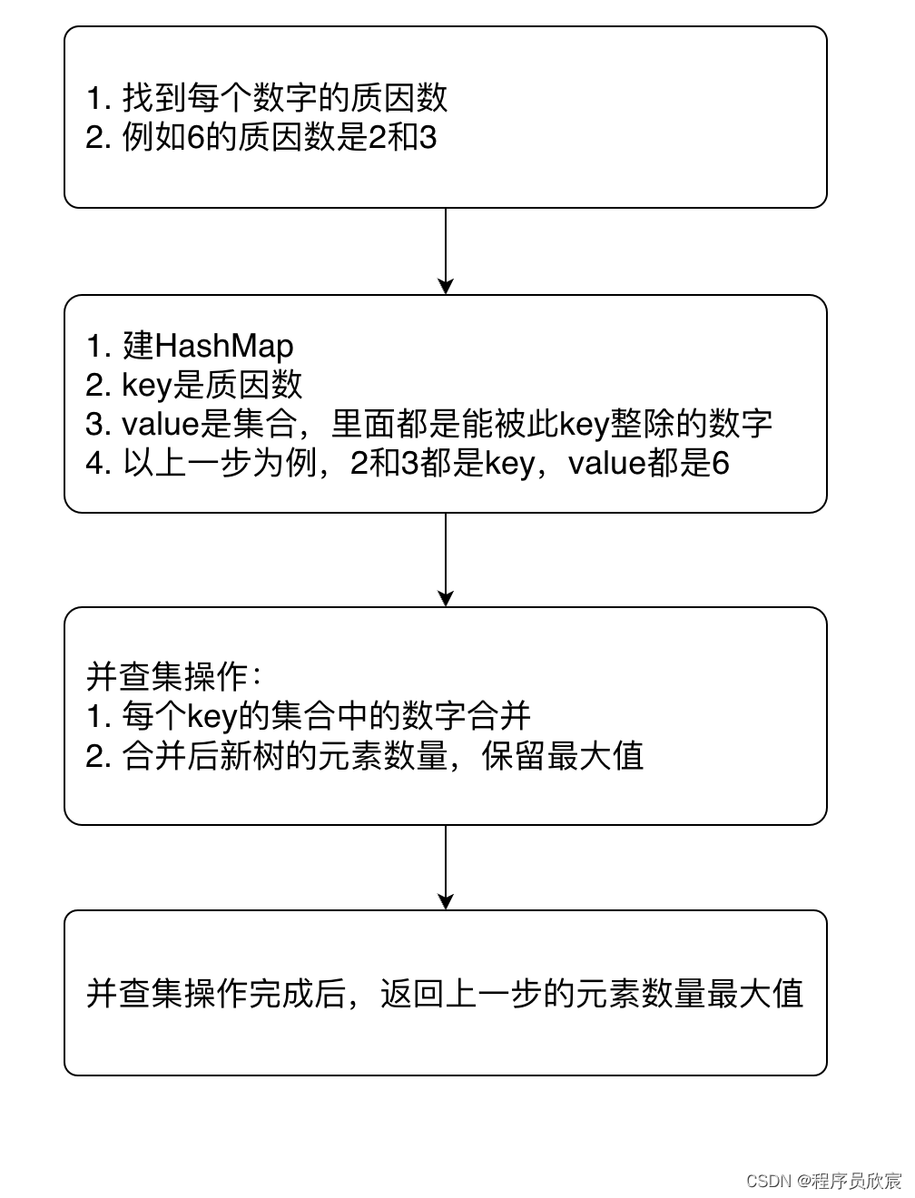
恒星的正方形问题

scikit-learn no moudule named six

number of solutions to solve a multivariate multi-degree equation

递归(各经典例题分析)

shell programming conventions and variables

程序员必备的 “ 摸鱼神器 ” 来了 !
随机推荐
Based on php animation peripheral mall management system (php graduation design)
_ _ determinant of a matrix is higher algebra eigenvalue of the product, the characteristic value of matrix trace is combined
SOM Network 2: Implementation of the Code
Based on php Xiangxi tourism website management system acquisition (php graduation design)
Anacoda的用途
number of solutions to solve a multivariate multi-degree equation
Safe fifth after-school exercise
迁移学习——Discriminative Transfer Subspace Learning via Low-Rank and Sparse Representation
Still struggling with reporting tool selection?To take a look at this
NFT的10种实际用途(NFT系统开发)
基于php动漫周边商城管理系统(php毕业设计)
威纶通触摸屏如何打开并升级EB8000旧版本项目并更换触摸屏型号?
Spark集群搭建
Mini Program--Independent Subcontracting & Subcontracting Pre-download
高等代数_证明_矩阵的任意特征值的代数重数大于等于其几何重数
【C语言实现】两种计算平均成绩题型,博主精心整理,值得一读
入门数据库Days4
小程序--分包
shell编程规范与变量
使用分类权重解决数据不平衡的问题