深度学习100例 —— 卷积神经网络(CNN)天气识别

活动地址：CSDN21天学习挑战赛

深度学习100例——卷积神经网络(CNN)天气识别

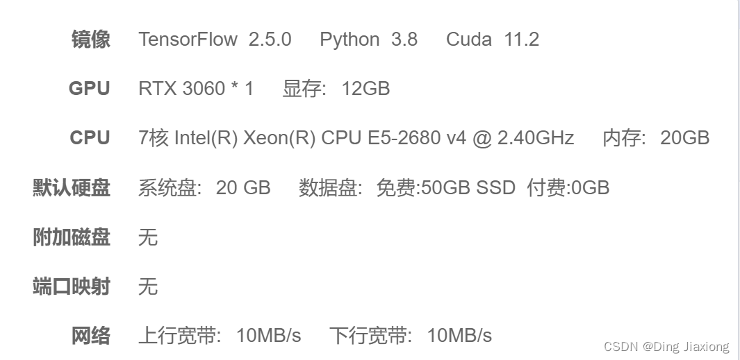
我的环境

1. 前期准备工作

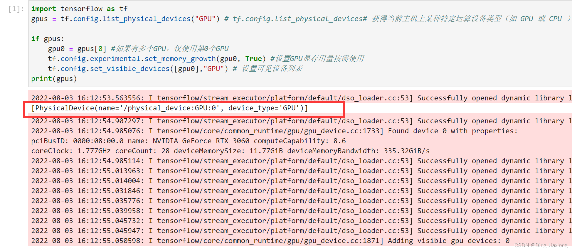
1.1 设置GPU

import tensorflow as tf
gpus = tf.config.list_physical_devices("GPU") # tf.config.list_physical_devices# 获得当前主机上某种特定运算设备类型（如 GPU 或 CPU ）的列表

if gpus:
    gpu0 = gpus[0] #如果有多个GPU，仅使用第0个GPU
    tf.config.experimental.set_memory_growth(gpu0, True) #设置GPU显存用量按需使用
    tf.config.set_visible_devices([gpu0],"GPU") # 设置可见设备列表

1.2 导入数据

import matplotlib.pyplot as plt
import os,PIL

# 设置随机种子尽可能使结果可以重现
import numpy as np
np.random.seed(1)

# 设置随机种子尽可能使结果可以重现
import tensorflow as tf
tf.random.set_seed(1)

from tensorflow import keras
from tensorflow.keras import layers,models

import pathlib

1.3 查看数据

数据集中一共有cloudy、rain、shine、sunrise四类。

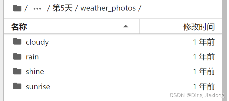
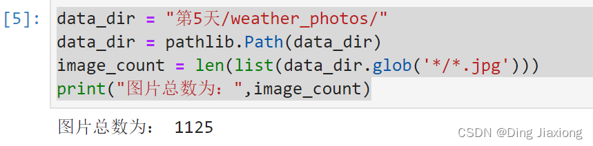
设置数据集路径及查看图片

data_dir = "第5天/weather_photos/"
data_dir = pathlib.Path(data_dir)
image_count = len(list(data_dir.glob('*/*.jpg')))
print("图片总数为：",image_count)

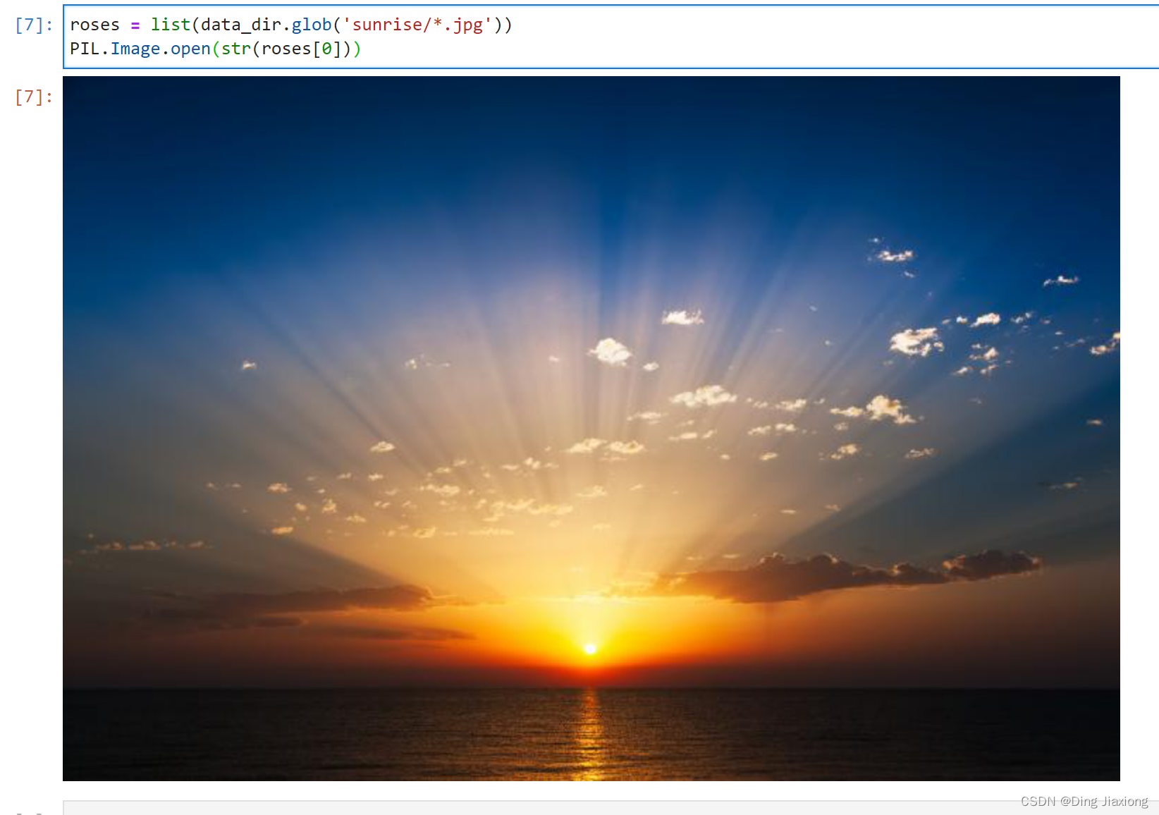
查看sunrise的第一张图片

roses = list(data_dir.glob('sunrise/*.jpg'))
PIL.Image.open(str(roses[0]))

2. 数据预处理

2.1 加载数据

使用image dataset_from directory方法将磁盘中的数据加载到tf.data.Dataset中

batch_size = 32 # 用于控制数据批次的大小，默认32
img_height = 180 # 图片像素高度
img_width = 180 # 图片像素宽度

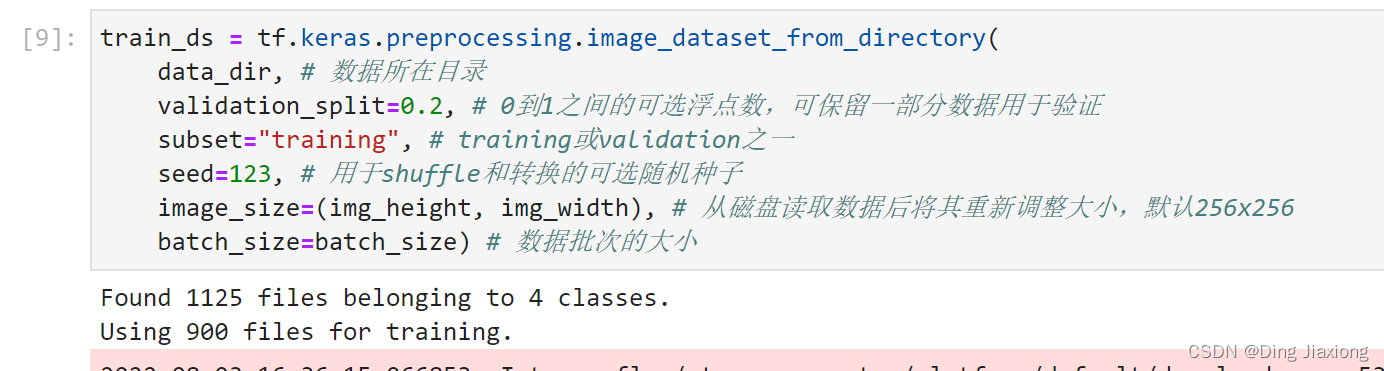
train_ds = tf.keras.preprocessing.image_dataset_from_directory(
    data_dir, # 数据所在目录
    validation_split=0.2, # 0到1之间的可选浮点数，可保留一部分数据用于验证
    subset="training", # training或validation之一
    seed=123, # 用于shuffle和转换的可选随机种子
    image_size=(img_height, img_width), # 从磁盘读取数据后将其重新调整大小，默认256x256
    batch_size=batch_size) # 数据批次的大小

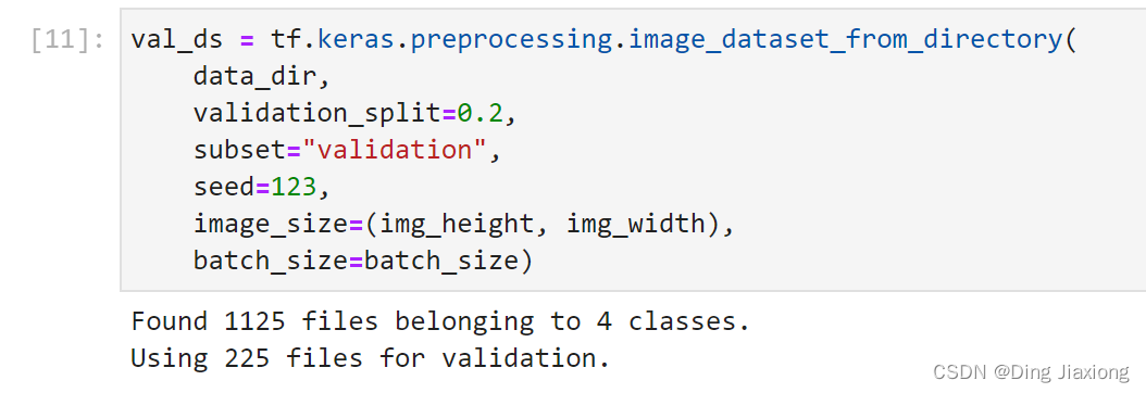
同样的设置验证数据集。

val_ds = tf.keras.preprocessing.image_dataset_from_directory(
    data_dir,
    validation_split=0.2,
    subset="validation",
    seed=123,
    image_size=(img_height, img_width),
    batch_size=batch_size)

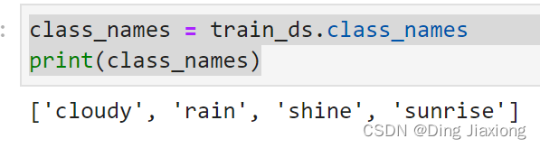
通过class_names输出数据集的标签，标签将按字母顺序对应于目录名称。

class_names = train_ds.class_names
print(class_names)

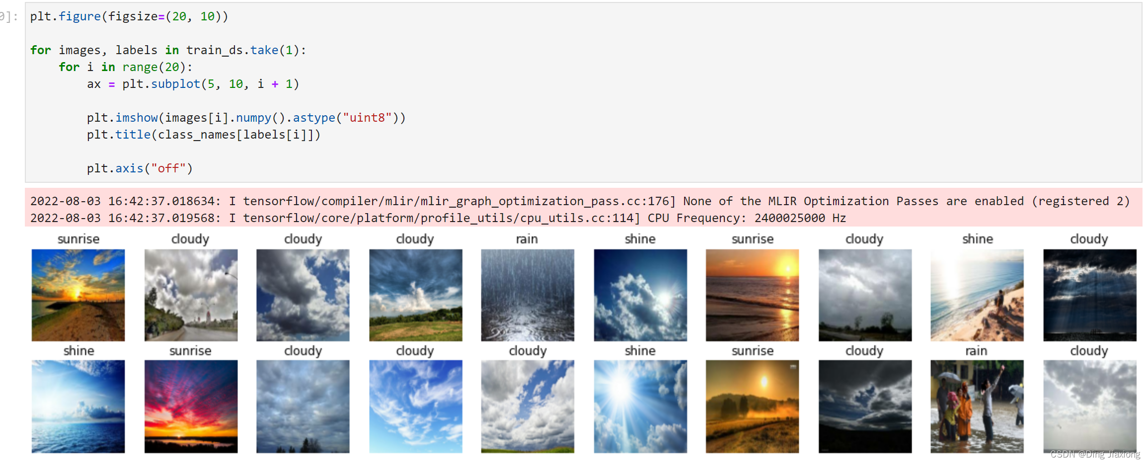
2.2 可视化数据

plt.figure(figsize=(20, 10))

for images, labels in train_ds.take(1):
    for i in range(20):
        ax = plt.subplot(5, 10, i + 1)

        plt.imshow(images[i].numpy().astype("uint8"))
        plt.title(class_names[labels[i]])
        
        plt.axis("off")

2.3 检查数据

for image_batch, labels_batch in train_ds:
    print(image_batch.shape)
    print(labels_batch.shape)
    break

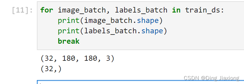
• image_batch是形状的张量(32 , 180 , 180 ,3)。3通道的180x180，32张图
• labels_batch是(32 , ) ， 对应32张图片

2.4 配置数据集

• shuffle()：打乱数据

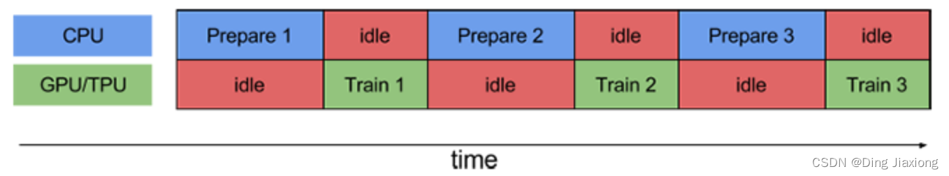
• prefetch()：预取数据，加速运行

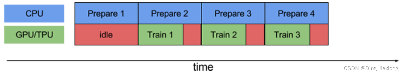
  CPU正在准备数据时，加速器处于空闲状态。相反，当加速器正在训练模型时，CPU处于空闲状态。因此，训练所用的时间是CPU预处理时间和加速器训练时间的总和。prefetch()将训练步骤的预处理和模型执行过程重叠到一起。当加速器正在执行第N个训练步时,CPU正在准备第N+1步的数据。这样做不仅可以最大限度地缩短训练的单步用时〈（而不是总用时)，而且可以缩短提取和转换数据所需的时间。如果不使用prefetch( )，CPU和GPU/TPU在大部分时间都处于空闲状态:

  

  使用prefetch()可以显著减少空闲时间：

  

• cache()：将数据集缓存到内存当中，加速运行

AUTOTUNE = tf.data.AUTOTUNE

train_ds = train_ds.cache().shuffle(1000).prefetch(buffer_size=AUTOTUNE)
val_ds = val_ds.cache().prefetch(buffer_size=AUTOTUNE)

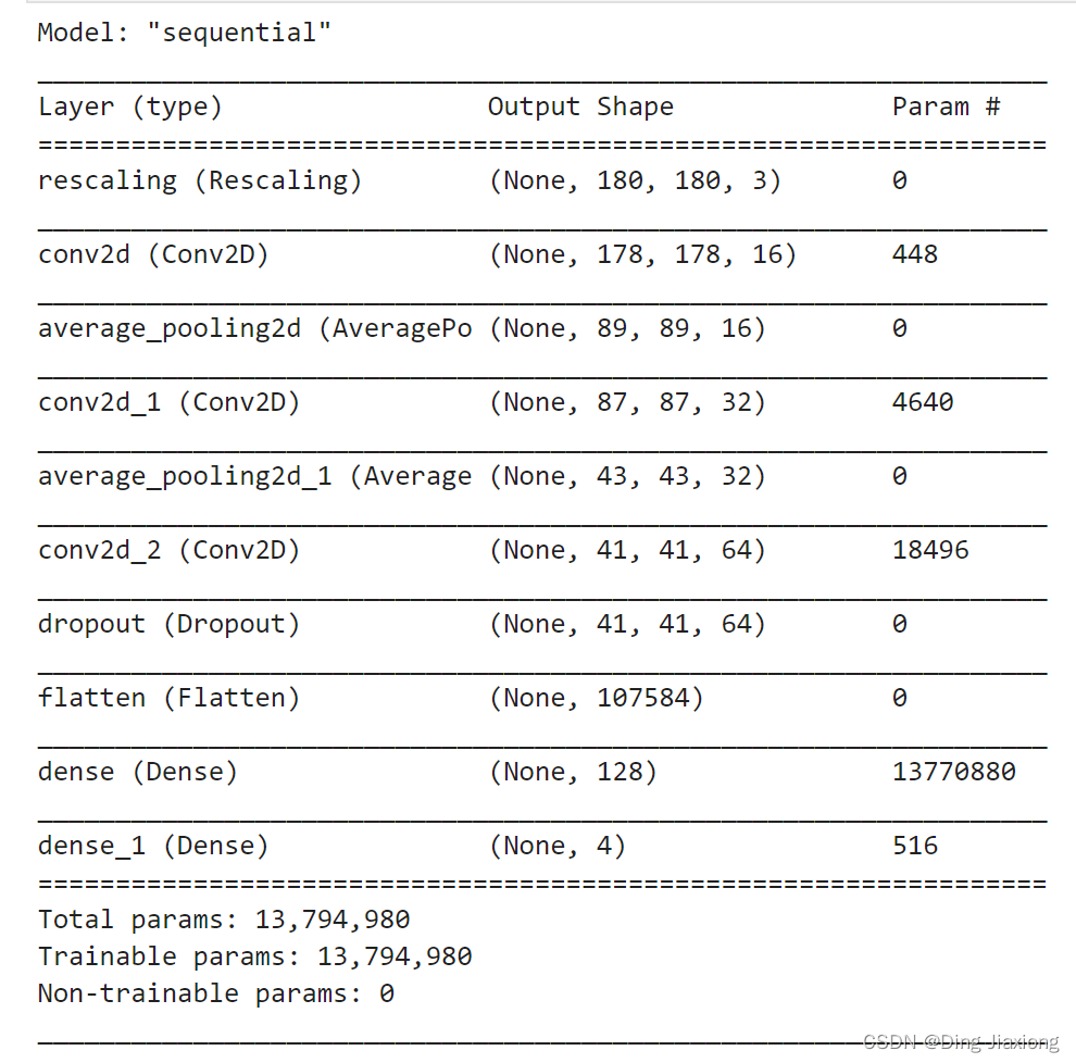
3. 构建CNN网络

num_classes = 4

model = models.Sequential([
    layers.experimental.preprocessing.Rescaling(1./255, input_shape=(img_height, img_width, 3)),
    
    layers.Conv2D(16, (3, 3), activation='relu', input_shape=(img_height, img_width, 3)), # 卷积层1，卷积核3*3 
    layers.AveragePooling2D((2, 2)),               # 池化层1，2*2采样
    layers.Conv2D(32, (3, 3), activation='relu'),  # 卷积层2，卷积核3*3
    layers.AveragePooling2D((2, 2)),               # 池化层2，2*2采样
    layers.Conv2D(64, (3, 3), activation='relu'),  # 卷积层3，卷积核3*3
    layers.Dropout(0.3),  
    
    layers.Flatten(),                       # Flatten层，连接卷积层与全连接层
    layers.Dense(128, activation='relu'),   # 全连接层，特征进一步提取
    layers.Dense(num_classes)               # 输出层，输出预期结果
])

model.summary()  # 打印网络结构

4. 编译模型

• 损失函数loss：用于衡量模型在训练期间的准确率
• 优化器optimizer：决定模型如何根据其看到的数据和自身的损失函数进行更新。
• 指标metrics：用于监控训练和测试步骤。

# 设置优化器
opt = tf.keras.optimizers.Adam(learning_rate=0.001)
model.compile(optimizer=opt,loss=tf.keras.losses.SparseCategoricalCrossentropy(from_logits=True),metrics=['accuracy'])

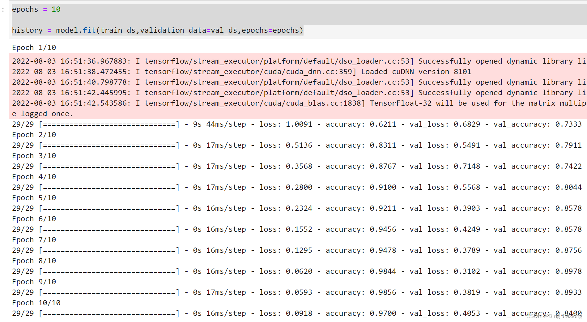
5. 训练模型

epochs = 10

history = model.fit(train_ds,validation_data=val_ds,epochs=epochs)

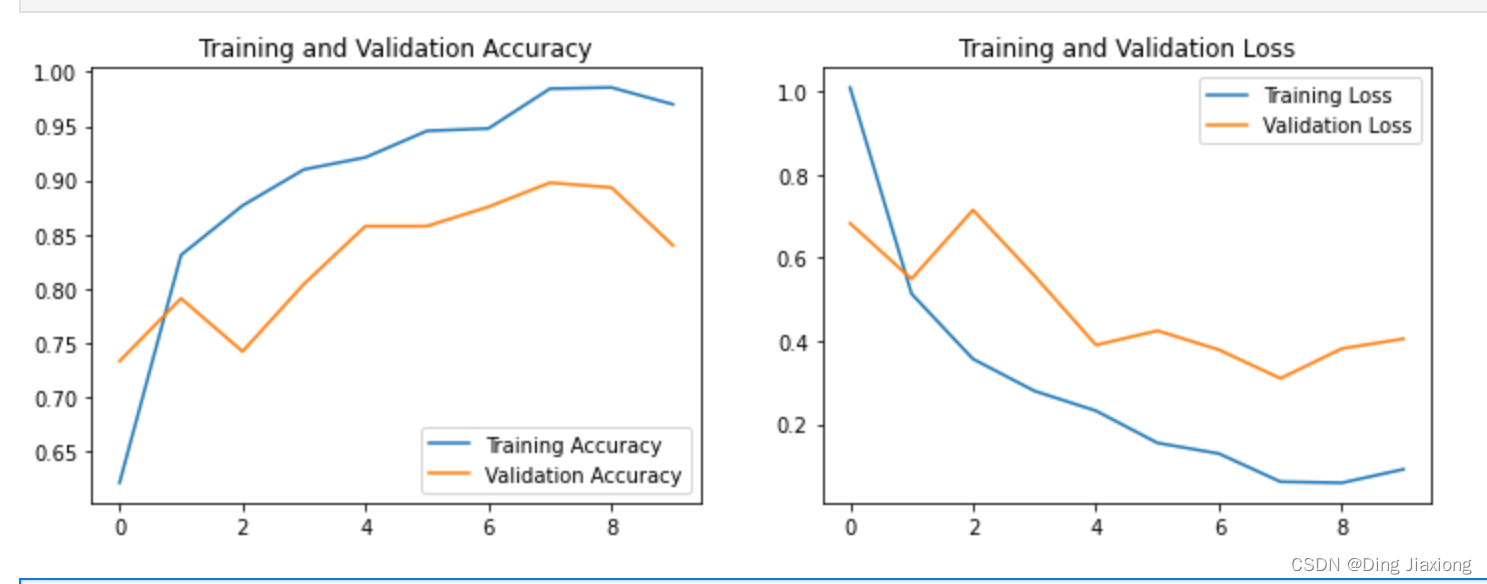
6. 模型评估

acc = history.history['accuracy']
val_acc = history.history['val_accuracy']

loss = history.history['loss']
val_loss = history.history['val_loss']

epochs_range = range(epochs)

plt.figure(figsize=(12, 4))
plt.subplot(1, 2, 1)
plt.plot(epochs_range, acc, label='Training Accuracy')
plt.plot(epochs_range, val_acc, label='Validation Accuracy')
plt.legend(loc='lower right')
plt.title('Training and Validation Accuracy')

plt.subplot(1, 2, 2)
plt.plot(epochs_range, loss, label='Training Loss')
plt.plot(epochs_range, val_loss, label='Validation Loss')
plt.legend(loc='upper right')
plt.title('Training and Validation Loss')
plt.show()