当前位置:网站首页>[secretly kill little buddy pytorch20 days -day02- example of image data modeling process]
[secretly kill little buddy pytorch20 days -day02- example of image data modeling process]
2022-07-03 20:53:00 【Can't write code】
It's today pytorch The second day of learning to punch in , come on. !!
Print the training time during the training
import os
import datetime

# Print time
def printbar():
    nowtime = datetime.datetime.now().strftime('%Y-%m-%d %H:%M:%S')
    print("\n"+"=========="*8 + "%s"%nowtime)
1. Prepare the data
cifar2 The data set is cifar10 A subset of a dataset , Only the first two categories are included airplane and automobile.
The training set has airplane and automobile Each picture 5000 Zhang , The test set has airplane and automobile Each picture 1000 Zhang .
cifar2 The goal of the mission is to train a model for the aircraft airplane And motor vehicles automobile Classify two kinds of pictures .
( If you need data set, please pay attention to private chat with me )
stay Pytorch There are usually two ways to build a picture data pipeline in .
The first is to use torchvision Medium datasets.ImageFolder To read the picture and then use DataLoader To load in parallel .
The second is through inheritance torch.utils.data.Dataset Implement user-defined read logic, and then use DataLoader To load in parallel .
The second method is a general method of reading user-defined data sets , You can read the picture data set , You can also read text data sets .
In this article, we introduce the first method .
import torch
from torch import nn
from torch.utils.data import Dataset,DataLoader
from torchvision import transforms,datasets

transform_train = transforms.Compose(
    [transforms.ToTensor()])
transform_valid = transforms.Compose(
    [transforms.ToTensor()])

ds_train = datasets.ImageFolder("cifar2/train",
            transform = transform_train,target_transform= lambda t:torch.tensor([t]).float())
ds_valid = datasets.ImageFolder("cifar2/test",
            transform = transform_train,target_transform= lambda t:torch.tensor([t]).float())

print(ds_train.class_to_idx)

Let's talk about it here ImageFolder
ImageFolder Suppose all files are saved in folders , Each folder stores pictures of the same category , The folder name is class name , The constructor is as follows :
ImageFolder(root, transform=None, target_transform=None, loader=default_loader)
It has four main parameters :
root: stay root Search for pictures in the specified path
transform: Yes PIL Image Conversion operation ,transform The input of is to use loader Read the return object of the picture
target_transform: Yes label Transformation
loader: How to read a picture after a given path , The default read is RGB Format PIL Image object
label It is sorted according to the folder name and saved as a dictionary , namely { Class name : Class No ( from 0 Start )}, In general, it's best to name the folder directly from 0 The starting number , This will be with ImageFolder Actually label Agreement , If not for this naming convention , Advice to see self.class_to_idx Attribute to understand label Mapping with folder name .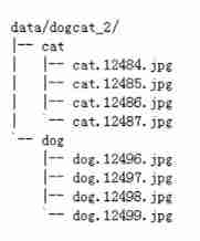
dl_train = DataLoader(ds_train,batch_size = 50,shuffle = True,num_workers=3)
dl_valid = DataLoader(ds_valid,batch_size = 50,shuffle = True,num_workers=3)
%matplotlib inline
%config InlineBackend.figure_format = 'svg'

# Check out some samples
from matplotlib import pyplot as plt

plt.figure(figsize=(8,8))
for i in range(9):
    img,label = ds_train[i]
    img = img.permute(1,2,0)
    ax=plt.subplot(3,3,i+1)
    ax.imshow(img.numpy())
    ax.set_title("label = %d"%label.item())
    ax.set_xticks([])
    ax.set_yticks([])
plt.show()

2. Defining models
Use Pytorch There are usually three ways to build models :
- Use nn.Sequential Build models in a hierarchical order ,
- Inherit nn.Module Base classes build custom models ,
- Inherit nn.Module Base classes build models and assist in applying model containers (nn.Sequential,nn.ModuleList,nn.ModuleDict) encapsulate .
Choose to inherit here nn.Module Base classes build custom models .
# test AdaptiveMaxPool2d The effect of
pool = nn.AdaptiveMaxPool2d((1,1))
t = torch.randn(10,8,32,32)
pool(t).shape
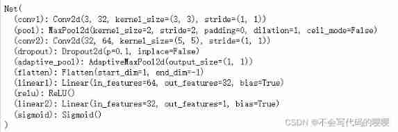
class Net(nn.Module):
def __init__(self):
super(Net, self).__init__()
self.conv1 = nn.Conv2d(in_channels=3,out_channels=32,kernel_size = 3)
self.pool = nn.MaxPool2d(kernel_size = 2,stride = 2)
self.conv2 = nn.Conv2d(in_channels=32,out_channels=64,kernel_size = 5)
self.dropout = nn.Dropout2d(p = 0.1)
self.adaptive_pool = nn.AdaptiveMaxPool2d((1,1))
self.flatten = nn.Flatten()
self.linear1 = nn.Linear(64,32)
self.relu = nn.ReLU()
self.linear2 = nn.Linear(32,1)
self.sigmoid = nn.Sigmoid()
def forward(self,x):
x = self.conv1(x)
x = self.pool(x)
x = self.conv2(x)
x = self.pool(x)
x = self.dropout(x)
x = self.adaptive_pool(x)
x = self.flatten(x)
x = self.linear1(x)
x = self.relu(x)
x = self.linear2(x)
y = self.sigmoid(x)
return y
net = Net()
print(net)
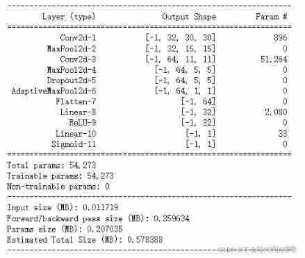
import torchkeras
torchkeras.summary(net,input_shape= (3,32,32))
3. Training models
Pytorch It usually requires the user to write a custom training cycle , The code style of the training cycle varies from person to person .
Yes 3 Class typical training cycle code style :
- Script form training cycle
- Function form training cycle
- Class form training cycle
Here we introduce a more general functional training cycle .
import pandas as pd
from sklearn.metrics import roc_auc_score

model = net
model.optimizer = torch.optim.SGD(model.parameters(),lr = 0.01)
model.loss_func = torch.nn.BCELoss()
model.metric_func = lambda y_pred,y_true: roc_auc_score(y_true.data.numpy(),y_pred.data.numpy())
model.metric_name = "auc"
def train_step(model,features,labels):

    #  Training mode ,dropout The layer acts
    model.train()

    #  Gradient clear
    model.optimizer.zero_grad()

    #  Forward propagation for loss
    predictions = model(features)
    loss = model.loss_func(predictions,labels)
    metric = model.metric_func(predictions,labels)

    #  Back propagation gradient
    loss.backward()
    model.optimizer.step()

    return loss.item(),metric.item()

def valid_step(model,features,labels):

    #  Prediction model ,dropout The layer does not work
    model.eval()
    #  Turn off gradient computation
    with torch.no_grad():
        predictions = model(features)
        loss = model.loss_func(predictions,labels)
        metric = model.metric_func(predictions,labels)

    return loss.item(), metric.item()


#  test train_step effect
features,labels = next(iter(dl_train))
train_step(model,features,labels)

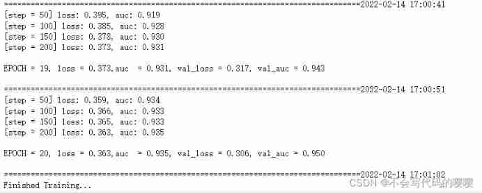
Start model training
def train_model(model,epochs,dl_train,dl_valid,log_step_freq):

    metric_name = model.metric_name
    dfhistory = pd.DataFrame(columns = ["epoch","loss",metric_name,"val_loss","val_"+metric_name])
    print("Start Training...")
    nowtime = datetime.datetime.now().strftime('%Y-%m-%d %H:%M:%S')
    print("=========="*8 + "%s"%nowtime)

    for epoch in range(1,epochs+1):

        # 1, Training cycle -------------------------------------------------
        loss_sum = 0.0
        metric_sum = 0.0
        step = 1

        for step, (features,labels) in enumerate(dl_train, 1):

            loss,metric = train_step(model,features,labels)

            #  Print batch The level of log
            loss_sum += loss
            metric_sum += metric
            if step%log_step_freq == 0:
                print(("[step = %d] loss: %.3f, "+metric_name+": %.3f") %
                      (step, loss_sum/step, metric_sum/step))

        # 2, Verification cycle -------------------------------------------------
        val_loss_sum = 0.0
        val_metric_sum = 0.0
        val_step = 1

        for val_step, (features,labels) in enumerate(dl_valid, 1):

            val_loss,val_metric = valid_step(model,features,labels)

            val_loss_sum += val_loss
            val_metric_sum += val_metric

        # 3, Log -------------------------------------------------
        info = (epoch, loss_sum/step, metric_sum/step,
                val_loss_sum/val_step, val_metric_sum/val_step)
        dfhistory.loc[epoch-1] = info

        #  Print epoch The level of log
        print(("\nEPOCH = %d, loss = %.3f,"+ metric_name + \
              " = %.3f, val_loss = %.3f, "+"val_"+ metric_name+" = %.3f")
              %info)
        nowtime = datetime.datetime.now().strftime('%Y-%m-%d %H:%M:%S')
        print("\n"+"=========="*8 + "%s"%nowtime)

    print('Finished Training...')

    return dfhistory
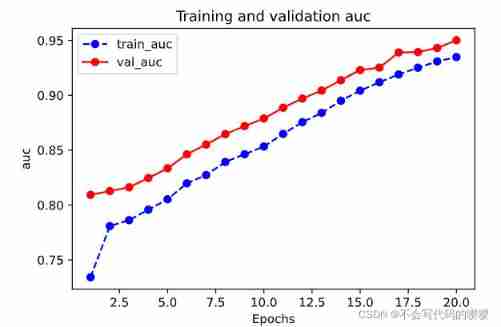
4. Model to evaluate
The evaluation of the model is generally to evaluate the effect on the training set and the verification set , During model training , We all keep one dfhistory Of , This is a DataFrame Structure , Inside is the change of the accuracy and loss of the model on the training set and the verification set during the training process , We can see the training of the model through visualization .
dfhistory

%matplotlib inline
%config InlineBackend.figure_format = 'svg'

import matplotlib.pyplot as plt

def plot_metric(dfhistory, metric):
    train_metrics = dfhistory[metric]
    val_metrics = dfhistory['val_'+metric]
    epochs = range(1, len(train_metrics) + 1)
    plt.plot(epochs, train_metrics, 'bo--')
    plt.plot(epochs, val_metrics, 'ro-')
    plt.title('Training and validation '+ metric)
    plt.xlabel("Epochs")
    plt.ylabel(metric)
    plt.legend(["train_"+metric, 'val_'+metric])
    plt.show()
plot_metric(dfhistory,"loss")

plot_metric(dfhistory,"auc")
5. Using the model
def predict(model,dl):
model.eval()
with torch.no_grad():
result = torch.cat([model.forward(t[0]) for t in dl])
return(result.data)
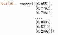
# Prediction probability
y_pred_probs = predict(model,dl_valid)
y_pred_probs
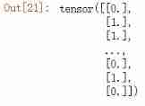
# Forecast category
y_pred = torch.where(y_pred_probs>0.5,
        torch.ones_like(y_pred_probs),torch.zeros_like(y_pred_probs))
y_pred
6. Save the model
It is recommended to save the parameters Pytorch Model .
#  Print related parameter names
print(model.state_dict().keys())

# Save model parameters
torch.save(model.state_dict(), "./data/model_parameter.pkl")
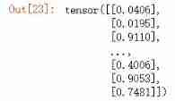
net_clone = Net()
net_clone.load_state_dict(torch.load("./data/model_parameter.pkl"))
predict(net_clone,dl_valid)
边栏推荐
- Cap and base theory
- AI enhanced safety monitoring project [with detailed code]
- Golang type assertion and conversion (and strconv package)
- 【leetcode】1027. Longest arithmetic sequence (dynamic programming)
- 2.2 integer
- QT6 QML book/qt quick 3d/ Basics
- 2.5 conversion of different data types (2)
- Redis data migration (II)
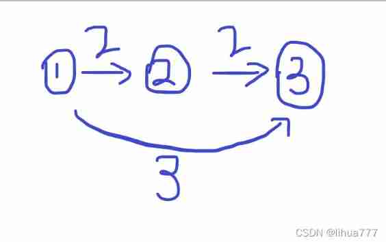
- Gauss elimination solves linear equations (floating-point Gauss elimination template)
- Q&A:Transformer, Bert, ELMO, GPT, VIT
猜你喜欢

Machine learning support vector machine SVM

内存分析器 (MAT)

It is discussed that the success of Vit lies not in attention. Shiftvit uses the precision of swing transformer to outperform the speed of RESNET

2022 safety officer-c certificate examination and safety officer-c certificate registration examination
Redis data migration (II)
Shortest path problem of graph theory (acwing template)

In 2021, the global foam protection packaging revenue was about $5286.7 million, and it is expected to reach $6615 million in 2028

Research Report on the overall scale, major manufacturers, major regions, products and application segmentation of rotary tablet presses in the global market in 2022

An old programmer gave it to college students
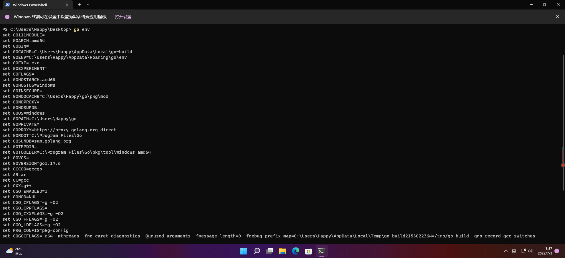
【愚公系列】2022年7月 Go教学课程 002-Go语言环境安装
随机推荐
Print linked list from end to end
Machine learning support vector machine SVM
MySQL learning notes - single table query
Transformation between yaml, Jason and Dict
Gauss elimination solves linear equations (floating-point Gauss elimination template)
Nmap and masscan have their own advantages and disadvantages. The basic commands are often mixed to increase output
How to choose cache read / write strategies in different business scenarios?
Etcd 基于Raft的一致性保证
(5) Web security | penetration testing | network security operating system database third-party security, with basic use of nmap and masscan
Last week's content review
Get log4net log file in C - get log4net log file in C
An old programmer gave it to college students
App compliance
How to do Taobao full screen rotation code? Taobao rotation tmall full screen rotation code
The 12th Blue Bridge Cup
Node MySQL serialize cannot rollback transactions
Basic preprocessing and data enhancement of image data
Instructions for common methods of regular expressions
MDM mass data synchronization test verification
It is discussed that the success of Vit lies not in attention. Shiftvit uses the precision of swing transformer to outperform the speed of RESNET