深蓝学院-视觉SLAM十四讲-第七章作业

第七节课作业

2. Bundle Adjustment

2.1 文献阅读

1. 为何说Bundle Adjustment is slow 是不对的？
   论文page 2，原文：The claimed slowness is almost always due to the unthinking use of a general-purpose optimization routine that completely ignores the problem structure and sparseness.
   在之前的文献中，BA一直被误认为是比较慢的，因为没有考虑到问题的结构和稀疏性。直接对$H$求逆来计算增量方程，会消耗很多计算资源，也就显得比较慢。实际上，由于$H$具有稀疏结构，是可以使用加速技巧进行求解的。而经过处理的BA，通常比其他新的方法更快，更有效。

2. BA 中有哪些需要注意参数化的地⽅？Pose 和Point 各有哪些参数化⽅式？有何优缺点。

   3D points（也就是路标点y）、3D Rotation（也就是相机外参数(R，t) 或者说是相机的位姿）、相机校准（camera calibration）也就是相机内参数 、投影后的像素坐标。

   Pose: 变换矩阵、欧拉角(Euler angles)、四元数(quaternions)

   欧拉角的优点是非常直观，缺点是容易产生万向锁问题

   变换矩阵的优点是描述方便，缺点是产生的参数过多，需要16个参数来描述变换过程。

   四元数的优点是计算方便，没有万向锁问题，缺点是理解起来比较困难、不直观。

   Point: 三维坐标点（X,Y,Z）、逆深度

   三维坐标点优点是比较简单直观，缺点是无法描述无限远的点；

   逆深度优点在于能够建模无穷远点；在实际应用中，逆深度也具有更好的数值稳定性。

   本题参考了文献的P7和博客：https://www.cnblogs.com/guoben/p/13375128.html

3. 本⽂写于2000 年，但是⽂中提到的很多内容在后⾯⼗⼏年的研究中得到了印证。你能看到哪些⽅向在后续⼯作中有所体现？请举例说明。

   • Intensity-based方法就是直接法的Bundle Adjustment;
   • 文中提的Network Structure对应现在应用比较广泛的图优化方式;
   • H的稀疏性可以实现BA实时，在07年的PTAM上实现。

2.2 BAL-dataset

本题参照了课本P257中g2o求解BA的例子，以及博客https://blog.csdn.net/QLeelq/article/details/115497273关于g2o的使用说明。

g2o的使用步骤大致为：

1. 创建一个线性求解器LinearSolver；
2. 创建BlockSolver，并用上面定义的线性求解器初始化；
3. 创建总求解器solver，并从GN/LM/DogLeg 中选一个作为迭代策略，再用上述块求解器BlockSolver初始化；
4. 创建图优化的核心：稀疏优化器（SparseOptimizer）；
5. 定义图的顶点和边，并添加到SparseOptimizer中；
6. 设置优化参数，开始执行优化。

BAL 的投影模型⽐教材中介绍的多了个负号，投影模型部分代码：

Vector2d project(const Vector3d &point) {
        //1.把世界坐标转换成像素坐标
        Vector3d pc = _estimate.rotation * point + _estimate.translation;
        //2.归一化坐标，BAL的投影模型比教材中介绍的多一个负号
        pc = -pc / pc[2];
        double r2 = pc.squaredNorm();
        //3.考虑归一化坐标的畸变模型
        double distortion = 1.0 + r2 * (_estimate.k1 + _estimate.k2 * r2);
        //4.根据内参模型计算像素坐标
        return Vector2d(_estimate.focal * distortion * pc[0],
                        _estimate.focal * distortion * pc[1]);
    }

路标点定义：

//继承并重写BaseVertex类，并实现接口
class VertexPoint : public g2o::BaseVertex<3, Vector3d> {
public:
    EIGEN_MAKE_ALIGNED_OPERATOR_NEW;

    VertexPoint() {}

    virtual void setToOriginImpl() override {
        _estimate = Vector3d(0, 0, 0);
    }

    virtual void oplusImpl(const double *update) override {
        _estimate += Vector3d(update[0], update[1], update[2]);
    }

    virtual bool read(istream &in) {}

    virtual bool write(ostream &out) const {}
};

投影边的定义：

//边的定义
class EdgeProjection :
    public g2o::BaseBinaryEdge<2, Vector2d, VertexPoseAndIntrinsics, VertexPoint> {
public:
    EIGEN_MAKE_ALIGNED_OPERATOR_NEW;

    virtual void computeError() override {
        auto v0 = (VertexPoseAndIntrinsics *) _vertices[0];
        auto v1 = (VertexPoint *) _vertices[1];
        auto proj = v0->project(v1->estimate());
        _error = proj - _measurement;
    }

    // use numeric derivatives
    virtual bool read(istream &in) {}

    virtual bool write(ostream &out) const {}

};

详细代码和编译文件在code文件夹下。选择problem-52-64053-pre.txt数据。

程序运行结果如下图所示，左边为初始图，右边为BA优化后的图：

3. 直接法的Bundle Adjustment

3.1 数学模型

1. 如何描述任意⼀点投影在任意⼀图像中形成的error？

$$error=I(p_i)-I_j(\pi (K{T}_J{p}_i))$$

2. 每个error 关联⼏个优化变量？

   关联两个优化变量，分别是位姿和路标点。也就是相机的李代数和三位空间坐标点P(x,y,z)。

3. error 关于各变量的雅可⽐是什么？

   本题与上一次课程作业的直接法中的误差相对于变量的雅克比求解类似。第二版课本P220。

   投影方程关于相机坐标系下的三维点的导数：
   $$\frac{\partial u}{\partial q}=\left[\begin{array}{ccc}\frac{f_x}{Z}& 0& -\frac{f_{x}X}{Z^2}\\ 0& \frac{f_y}{Z}& -\frac{f_{y}Y}{Z^2}\end{array}\right]$$
   变换后的三维点对变换的导数：
   $$\frac{\partial q}{\partial \delta \xi }=\left[\begin{array}{cc}I,& -q^{\wedge }\end{array}\right]$$
   其中两项可以合并得：
   $$\frac{\partial u}{\partial q}\cdot \frac{\partial q}{\partial \delta \xi }=\frac{\partial u}{\partial \delta \xi }=\left[\begin{array}{ccccccc}\frac{f_x}{Z}& 0& -\frac{f_{x}X}{Z^2}& -\frac{f_{x}XY}{Z^2}& f_x+\frac{f_x{X}^2}{Z^2}& -\frac{f_{x}Y}{Z}& \\ 0& \frac{f_y}{Z}& -\frac{f_{y}Y}{Z^2}& -f_y-\frac{f_y{Y}^2}{Z^2}& \frac{f_{y}XY}{Z^2}& \frac{f_{y}X}{Z}& \end{array}\right]$$
   误差相对于李代数的雅克比：
   $$J=-\frac{\partial I_2}{\partial u}\frac{\partial u}{\partial \delta \xi }$$
   误差相对于3D坐标点的雅克比：
   $$J=-\frac{\partial I_2}{\partial u}\frac{\partial u}{\partial P}$$

3.2 实现

1. 能否不要以[x; y; z]T 的形式参数化每个点？

​ 可以，还可以使用逆深度的方法来参数化每个点，这种方式可以表示无限远点。

2. 取4x4 的patch 好吗？取更⼤的patch 好还是取⼩⼀点的patch 好？

​ 4*4的patch应该是一个比较适中的大小，patch过大会导致计算量大，过小则会导致鲁棒性不强。

3. 从本题中，你看到直接法与特征点法在BA 阶段有何不同？

​ 最大的不同就是误差的计算不同，直接法计算的是光度误差，特征点法计算的是重投影误差。

4. 由于图像的差异，你可能需要鲁棒核函数，例如Huber。此时Huber 的阈值如何选取？

​ Huber阈值应该是根据多次实验，按照经验来确定的。

计算误差：

 // TODO START YOUR CODE HERE
        const g2o::VertexPointXYZ *vertexPw = static_cast<const g2o::VertexPointXYZ * >(vertex(0));
        const VertexSophus *vertexTcw = static_cast<const VertexSophus * >(vertex(1));
        Eigen::Vector3d Pc = vertexTcw->estimate() * vertexPw->estimate();
        float u = Pc[0] / Pc[2] * fx + cx;
        float v = Pc[1] / Pc[2] * fy + cy;
        if (u - 2 < 0 || v - 2 <0 || u+1 >= targetImg.cols || v + 1 >= targetImg.rows) {
            //边界点的处理(error设为0，setLevel(1))
            this->setLevel(1);
            for (int n = 0; n < 16; n++)
                _error[n] = 0;
        } else {
            for (int i = -2; i < 2; i++) {
                for (int j = -2; j < 2; j++) {
                    int num = 4 * i + j + 10;
                    _error[num] = origColor[num] - GetPixelValue(targetImg, u + i, v + j);
                }
            }
        }
// END YOUR CODE HERE

计算雅克比：

virtual void linearizeOplus() override {
        if (level() == 1) {
            _jacobianOplusXi = Eigen::Matrix<double, 16, 3>::Zero();
            _jacobianOplusXj = Eigen::Matrix<double, 16, 6>::Zero();
            return;
        }
        const g2o::VertexPointXYZ *vertexPw = static_cast<const g2o::VertexPointXYZ * >(vertex(0));
        const VertexSophus *vertexTcw = static_cast<const VertexSophus * >(vertex(1));
        Eigen::Vector3d Pc = vertexTcw->estimate() * vertexPw->estimate();
        float x = Pc[0];
        float y = Pc[1];
        float z = Pc[2];
        float inv_z = 1.0 / z;
        float inv_z2 = inv_z * inv_z;
        float u = x * inv_z * fx + cx;
        float v = y * inv_z * fy + cy;

        Eigen::Matrix<double, 2, 3> J_Puv_Pc;
        J_Puv_Pc(0, 0) = fx * inv_z;
        J_Puv_Pc(0, 1) = 0;
        J_Puv_Pc(0, 2) = -fx * x * inv_z2;
        J_Puv_Pc(1, 0) = 0;
        J_Puv_Pc(1, 1) = fy * inv_z;
        J_Puv_Pc(1, 2) = -fy * y * inv_z2;

        Eigen::Matrix<double, 3, 6> J_Pc_kesi = Eigen::Matrix<double, 3, 6>::Zero();
        J_Pc_kesi(0, 0) = 1;
        J_Pc_kesi(0, 4) = z;
        J_Pc_kesi(0, 5) = -y;
        J_Pc_kesi(1, 1) = 1;
        J_Pc_kesi(1, 3) = -z;
        J_Pc_kesi(1, 5) = x;
        J_Pc_kesi(2, 2) = 1;
        J_Pc_kesi(2, 3) = y;
        J_Pc_kesi(2, 4) = -x;

        Eigen::Matrix<double, 1, 2> J_I_Puv;
        for (int i = -2; i < 2; i++)
            for (int j = -2; j < 2; j++) {
                int num = 4 * i + j + 10;
                J_I_Puv(0, 0) =
                        (GetPixelValue(targetImg, u + i + 1, v + j) - GetPixelValue(targetImg, u + i - 1, v + j)) / 2;
                J_I_Puv(0, 1) =
                        (GetPixelValue(targetImg, u + i, v + j + 1) - GetPixelValue(targetImg, u + i, v + j - 1)) / 2;
                _jacobianOplusXi.block<1, 3>(num, 0) = -J_I_Puv * J_Puv_Pc * vertexTcw->estimate().rotationMatrix();
                _jacobianOplusXj.block<1, 6>(num, 0) = -J_I_Puv * J_Puv_Pc * J_Pc_kesi;
            }
    }

构建BA问题：

    // build optimization problem
    typedef g2o::BlockSolver<g2o::BlockSolverTraits<6, 3>> DirectBlock;  // 求解的向量是6＊1的
    std::unique_ptr<DirectBlock::LinearSolverType> linearSolver ( new g2o::LinearSolverDense<DirectBlock::PoseMatrixType>()); // 线性方程求解器
    std::unique_ptr<DirectBlock> solver_ptr ( new DirectBlock ( std::move(linearSolver)));     // 矩阵块求解器
    g2o::OptimizationAlgorithmLevenberg* solver = new g2o::OptimizationAlgorithmLevenberg ( std::move(solver_ptr));  //选择使用LM优化 

    g2o::SparseOptimizer optimizer;
    optimizer.setAlgorithm(solver);
    optimizer.setVerbose(true);

    // TODO add vertices, edges into the graph optimizer
    // START YOUR CODE HERE
    for (int k = 0; k < points.size(); ++k) {
        g2o::VertexPointXYZ* pPoint = new g2o::VertexPointXYZ();
        pPoint->setId(k);
        pPoint->setEstimate(points[k]);
        pPoint->setMarginalized(true);//使用稀疏优化时手动设置需要边缘化的顶点 优化目标仅为位姿结点,所以路标结点需要边缘化
        optimizer.addVertex(pPoint);
    }
    for (int j = 0; j < poses.size(); j++) {
        VertexSophus *vertexTcw = new VertexSophus();
        vertexTcw->setEstimate(poses[j]);
        // 两种节点的id顺序保持连续
        vertexTcw->setId(j + points.size());
        optimizer.addVertex(vertexTcw);
    }
    for (int c = 0; c < poses.size(); c++)
        for (int p = 0; p < points.size(); p++) {
            EdgeDirectProjection *edge = new EdgeDirectProjection(color[p], images[c]);
            // 先point后pose
            edge->setVertex(0, dynamic_cast<g2o::VertexPointXYZ *>(optimizer.vertex(p)));
            edge->setVertex(1, dynamic_cast<VertexSophus *>(optimizer.vertex(c + points.size())));
            // 信息矩阵可直接设置为 error_dim*error_dim 的单位阵
            edge->setInformation(Eigen::Matrix<double, 16, 16>::Identity());
            //　设置Huber核函数，减小错误点影响，加强鲁棒性
            g2o::RobustKernelHuber *rk = new g2o::RobustKernelHuber;
            rk->setDelta(1.0);
            edge->setRobustKernel(rk);
            optimizer.addEdge(edge);
        }
// END YOUR CODE HERE

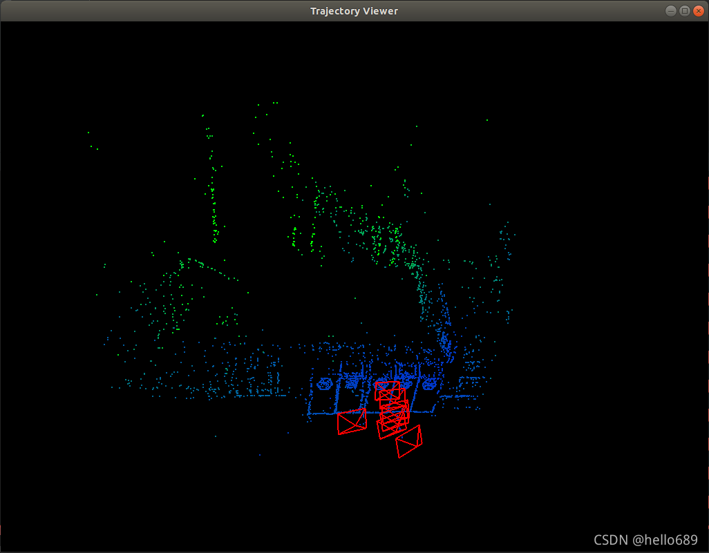
程序运行结果如下图所示：

优化前的位姿和点云：

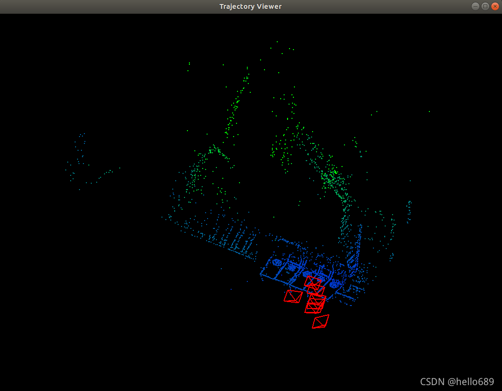
优化后的位姿和点云：

国内gitee地址：https://gitee.com/ximing689/slam-learning.git
github地址: https://github.com/ximing1998/slam-learning.git