当前位置:网站首页>Performance analysis of continuous time system (1) - performance index and first and second order analysis of control system
Performance analysis of continuous time system (1) - performance index and first and second order analysis of control system
2022-07-27 19:04:00 【Miracle Fan】
Self control principle learning notes
Self control principle learning notes column
List of articles
Preface
In control theory , The analysis of control system can be divided into time domain analysis and frequency domain analysis . Frequency domain analysis is by inputting sinusoidal input signals of different frequencies to the system , Analyze the steady-state response of the system ; Time domain analysis is to evaluate the performance of the system by studying the time response of the system . This chapter mainly studies the time domain performance and frequency domain performance of the system , Time domain response is to find out the specific response waveform of the system , Frequency analysis can only get the characteristic information of the system response .
1. Control system performance index

1.1 Transient performance
1.1.1 Rise time t r t_r tr——rise time
Steady state values range from 10%——>90% Time required ; Underdamped :0100%, Overdamping :1090%
1.1.2 Peak time t p t_p tp——peak time
The first peak time when the response reaches the overshoot
1.1.3 Maximum overshoot M p M_p Mp——maximum percent overshoot
Percentage of the final value exceeded for the first time
M p = y ( t p ) − y ( ∞ ) y ( ∞ ) × 100 % Non zero case : M p = y ( t p ) − y ( ∞ ) y ( ∞ ) − y ( 0 ) × 100 % M_p=\frac{y(t_p)-y(\infty)}{y(\infty)}\times100\%\\ {\color{Red} \text{ Non zero case :}M_p=\frac{y(t_p)-y(\infty)}{y(\infty)-y(0)}\times100\%} Mp=y(∞)y(tp)−y(∞)×100% Non zero case :Mp=y(∞)−y(0)y(tp)−y(∞)×100%
Generally, the faster the response , The greater the overshoot .
1.1.4 Adjust the time t s t_s ts——settling time
When the steady-state allowable error reaches 2 % ∼ 5 % 2\% \sim5\% 2%∼5%
1.1.5 Delay time t d t_d td——delay time
The response curve reaches 1 2 \frac{1}{2} 21 The time required for the steady-state value of
1.1.6 Number of oscillations
1.1.7 Attenuation ratio
1.2 Steady state performance
1.2.1 Steady state error —— e s s e_{ss} ess
The error between the actual value and the expected value of the steady-state response of the steady-state system .
2. Typical first-order time domain analysis
2.1 Definition
The typical first-order system block diagram can be simplified as follows .

structure characteristics :
- Unit negative feedback
- Open loop transfer function is another integral link , The open-loop gain is the reciprocal of the time constant K = 1 T K=\frac{1}{T} K=T1
2.2 Response of typical links
Unit step response - r ( t ) = ϵ ( t ) , R ( s ) = 1 s r(t)=\epsilon(t),R(s)=\frac{1}{s} r(t)=ϵ(t),R(s)=s1
Output is :
y ( t ) = 1 − e − t T → 1 e s s = lim t → ∞ e ( t ) = 0 y(t)=1-\mathrm{e}^{-\frac{t}{T}} \rightarrow 1\\ e_{ss}=\lim_{t\rightarrow\infty}e(t)=0 y(t)=1−e−Tt→1ess=t→∞lime(t)=0
The steady-state error is :Unit impulse response - r ( t ) = δ ( t ) , R ( s ) = 1 r(t)=\delta(t),R(s)=1 r(t)=δ(t),R(s)=1
Output is :
y ( t ) = 1 T e − t / T → 0 y(t)=\frac{1}{T} \mathrm{e}^{-t / T} \rightarrow 0\\ y(t)=T1e−t/T→0
The steady-state error is :
e ( t ) = r ( t ) − y ( t ) = δ ( t ) − T e − 1 T t e s s = lim t → ∞ e ( t ) = δ ( t ) − T e(t)=r(t)-y(t)=\delta(t)-Te^{-\frac{1}{T}t}\\ e_{ss}=\lim_{t\rightarrow\infty}e(t)=\delta(t)-T e(t)=r(t)−y(t)=δ(t)−Te−T1tess=t→∞lime(t)=δ(t)−TUnit slope response - r ( t ) = t , R ( s ) = 1 s 2 r(t)=t,R(s)=\frac{1}{s^2} r(t)=t,R(s)=s21
Output is :
y ( t ) = t − T + T e − t / T → t − T y(t)=t-T+T \mathrm{e}^{-t / T} \rightarrow t-T\\ y(t)=t−T+Te−t/T→t−T
Steady state error :
e ( t ) = r ( t ) − y ( t ) = T ( 1 − e − 1 T t ) e s s = lim t → ∞ e ( t ) = T e(t)=r(t)-y(t)=T(1-e^{-\frac{1}{T}t})\\ e_{ss}=\lim_{t\rightarrow\infty}e(t)=T e(t)=r(t)−y(t)=T(1−e−T1t)ess=t→∞lime(t)=TUnit acceleration response - r ( t ) = 1 2 t 2 , R ( s ) = 1 s 3 r(t)=\frac{1}{2}t^2,R(s)=\frac{1}{s^3} r(t)=21t2,R(s)=s31
Output is :
y ( t ) = 1 2 t 2 − T t + T 2 ( 1 − e − 1 T t ) → 1 2 t 2 − T t + T 2 y(t)=\frac{1}{2} t^{2}-T t+T^{2}\left(1-\mathrm{e}^{-\frac{1}{T} t}\right) \rightarrow \frac{1}{2} t^{2}-T t+T^{2} y(t)=21t2−Tt+T2(1−e−T1t)→21t2−Tt+T2
Steady state error :
e ( t ) = r ( t ) − y ( t ) = T t − T 2 ( 1 − e − 1 T t ) e s s = lim t → ∞ e ( t ) = ∞ e(t)=r(t)-y(t)=Tt-T^2(1-e^{-\frac{1}{T}t})\\ e_{ss}=\lim_{t\rightarrow\infty}e(t)=\infty e(t)=r(t)−y(t)=Tt−T2(1−e−T1t)ess=t→∞lime(t)=∞
The following figure shows the unit impulse response , Unit step response , Response function of unit slope response , You can see that the unit responds to each link by presenting integral / Differential relation , Then their output has also been integrated / Differential link .

3. Typical second-order time domain analysis
3.1 Definition
Transfer function :
Y ( s ) R ( s ) = ω n 2 s 2 + 2 ζ ω n s + ω n 2 \frac{Y(s)}{R(s)}=\frac{\omega_{\mathrm{n}}^{2}}{s^{2}+2 \zeta \omega_{\mathrm{n}} s+\omega_{\mathrm{n}}^{2}} R(s)Y(s)=s2+2ζωns+ωn2ωn2Typical structure diagram :

Structural features :
(1) Unit negative feedback structure
(2) The open-loop transfer function has only one integral link , The open-loop gain is K = w n / ( 2 ζ ) K=w_n/(2\zeta) K=wn/(2ζ)
3.2 Response of typical links
Slope response
Output is :
Y ( s ) = 1 s 2 ⋅ ω n 2 s 2 + 2 ζ ω n s + ω n 2 Y(s)=\frac{1}{s^{2}} \cdot \frac{\omega_{\mathrm{n}}^{2}}{s^{2}+2 \zeta \omega_{\mathrm{n}} s+\omega_{\mathrm{n}}^{2}} Y(s)=s21⋅s2+2ζωns+ωn2ωn2
Steady state error :
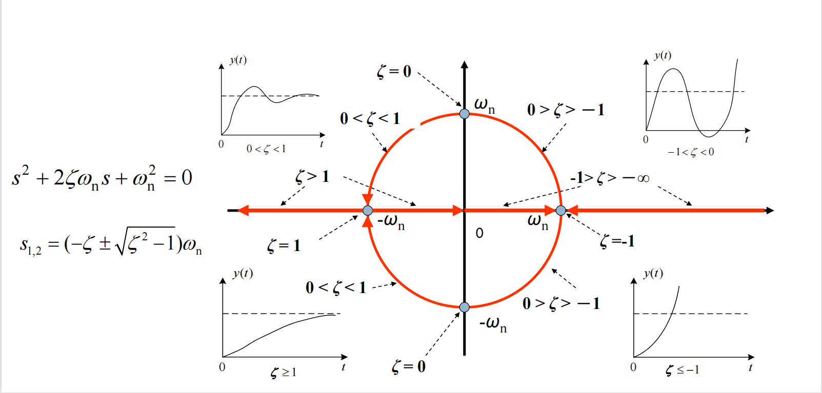
E ( s ) = R ( s ) − Y ( s ) = 1 s 2 − 1 s 2 ⋅ ω n 2 s 2 + 2 ζ ω n s + ω n 2 = 1 s ⋅ s + 2 ζ ω n s 2 + 2 ζ ω n s + ω n 2 e s s = lim t → ∞ e ( t ) = lim s → 0 s E ( s ) = lim s → 0 s + 2 ζ ω n s 2 + 2 ζ ω n s + ω n 2 = 2 ζ ω n \begin{aligned} E(s) &=R(s)-Y(s)=\frac{1}{s^{2}}-\frac{1}{s^{2}} \cdot \frac{\omega_{\mathrm{n}}^{2}}{s^{2}+2 \zeta \omega_{\mathrm{n}} s+\omega_{\mathrm{n}}^{2}} \\ &=\frac{1}{s} \cdot \frac{s+2 \zeta \omega_{\mathrm{n}}}{s^{2}+2 \zeta \omega_{\mathrm{n}} s+\omega_{\mathrm{n}}^{2}} \\ e_{ss}=\lim _{t \rightarrow \infty} e(t) &=\lim _{s \rightarrow 0} s E(s)=\lim _{s \rightarrow 0} \frac{s+2 \zeta \omega_{\mathrm{n}}}{s^{2}+2 \zeta \omega_{\mathrm{n}} s+\omega_{\mathrm{n}}^{2}}=\frac{2 \zeta}{\omega_{\mathrm{n}}} \end{aligned} E(s)ess=t→∞lime(t)=R(s)−Y(s)=s21−s21⋅s2+2ζωns+ωn2ωn2=s1⋅s2+2ζωns+ωn2s+2ζωn=s→0limsE(s)=s→0lims2+2ζωns+ωn2s+2ζωn=ωn2ζThe relationship between transient performance and damping coefficient and natural frequency angular frequency
ζ > 1 \zeta>1 ζ>1: Overdamping
ζ = 1 \zeta=1 ζ=1: Critical damping
0 < ζ < 1 0<\zeta<1 0<ζ<1: Underdamped , It has good transient performance , Attenuated oscillation .
4. Underdamped transient performance
4.1 Take the unit step response as an example :
Y ( s ) = 1 s ⋅ ω n 2 s 2 + 2 ζ ω n s + ω n 2 = 1 s − s + ζ ω n ( s + ζ ω n ) 2 + ( 1 − ζ 2 ) ω n 2 − ζ ( s + ζ ω n ) 2 + ( 1 − ζ 2 ) ω n 2 \begin{aligned} Y(s) =&\frac{1}{s} \cdot \frac{\omega_{\mathrm{n}}^{2}}{s^{2}+2 \zeta \omega_{\mathrm{n}} s+\omega_{\mathrm{n}}^{2}} \\ = & \frac{1}{s}-\frac{s+\zeta \omega_{\mathrm{n}}}{\left(s+\zeta \omega_{\mathrm{n}}\right)^{2}+\left(1-\zeta^{2}\right) \omega_{\mathrm{n}}^{2}}-\frac{\zeta}{\left(s+\zeta \omega_{\mathrm{n}}\right)^{2}+\left(1-\zeta^{2}\right) \omega_{\mathrm{n}}^{2}} \\ \end{aligned} Y(s)==s1⋅s2+2ζωns+ωn2ωn2s1−(s+ζωn)2+(1−ζ2)ωn2s+ζωn−(s+ζωn)2+(1−ζ2)ωn2ζ
y ( t ) = 1 − e − ζ ω n t [ cos ( 1 − ζ 2 ω n t ) + ζ 1 − ζ 2 sin ( 1 − ζ 2 ω n t ) ] = 1 − e − ζ ω n t 1 − ζ 2 [ 1 − ζ 2 cos ( 1 − ζ 2 ω n t ) + ζ sin ( 1 − ζ 2 ω n t ) ] = 1 − e − ζ ω n t 1 − ζ 2 [ sin ( arccos ζ ) cos ( 1 − ζ 2 ω n t ) + cos ( arccos ζ ) sin ( 1 − ζ 2 ω n t = 1 − e − ζ ω n t 1 − ζ 2 sin ( 1 − ζ 2 ω n t + arccos ζ ) \begin{aligned} y(t)&=1-\mathrm{e}^{-\zeta \omega_{\mathrm{n}} t}\left[\cos \left(\sqrt{1-\zeta^{2}} \omega_{\mathrm{n}} t\right)+\frac{\zeta}{\sqrt{1-\zeta^{2}}} \sin \left(\sqrt{1-\zeta^{2}} \omega_{\mathrm{n}} t\right)\right] \\ &=1-\frac{\mathrm{e}^{-\zeta \omega_{\mathrm{n}} t}}{\sqrt{1-\zeta^{2}}}\left[\sqrt{1-\zeta^{2}} \cos \left(\sqrt{1-\zeta^{2}} \omega_{\mathrm{n}} t\right)+\zeta \sin \left(\sqrt{1-\zeta^{2}} \omega_{\mathrm{n}} t\right)\right] \\ &=1-\frac{\mathrm{e}^{-\zeta \omega_{\mathrm{n}} t}}{\sqrt{1-\zeta^{2}}}\left[\sin (\arccos \zeta) \cos \left(\sqrt{1-\zeta^{2}} \omega_{\mathrm{n}} t\right)+\cos (\arccos \zeta) \sin \left(\sqrt{1-\zeta^{2} \omega_{\mathrm{n}} t}\right.\right. \\ &=1-\frac{\mathrm{e}^{-\zeta \omega_{\mathrm{n}} t}}{\sqrt{1-\zeta^{2}}} \sin \left(\sqrt{1-\zeta^{2}} \omega_{\mathrm{n}} t+\arccos \zeta\right) \\ \end{aligned} y(t)=1−e−ζωnt[cos(1−ζ2ωnt)+1−ζ2ζsin(1−ζ2ωnt)]=1−1−ζ2e−ζωnt[1−ζ2cos(1−ζ2ωnt)+ζsin(1−ζ2ωnt)]=1−1−ζ2e−ζωnt[sin(arccosζ)cos(1−ζ2ωnt)+cos(arccosζ)sin(1−ζ2ωnt=1−1−ζ2e−ζωntsin(1−ζ2ωnt+arccosζ)
remember failure reduce system Count σ = ζ w n , Resistance Ni Vibration Swing frequency rate w d = 1 − ζ 2 w n , cos β = ζ , sin β = 1 − ζ 2 , Its in β call by Resistance Ni horn Record the attenuation coefficient \sigma=\zeta w_n, Damped oscillation frequency w_d=\sqrt {1-\zeta^2}w_n,\cos\beta=\zeta,\sin\beta=\sqrt{1-\zeta^2}, among \beta This is called the damping angle remember failure reduce system Count σ=ζwn, Resistance Ni Vibration Swing frequency rate wd=1−ζ2wn,cosβ=ζ,sinβ=1−ζ2, Its in β call by Resistance Ni horn
4.2 Transient performance index
Peak time
Make y ˙ ( t ) = 0 , namely e − σ t ω n 1 − ζ 2 sin ( ω d t ) = 0 have to To : t = k π ω d , k = 1 , 2 , ⋯ The first One individual peak value Of when between by t p = π ω d = π ω n 1 − ζ 2 \begin{aligned} Make \dot{y}(t) & = 0 , namely \\ &\frac{\mathrm{e}^{-\sigma t} \omega_{\mathrm{n}}}{\sqrt{1-\zeta^{2}}} \sin \left(\omega_{\mathrm{d}} t\right) = 0\\ obtain :\\ &t = \frac{k \pi}{\omega_{d}}, k = 1,2, \cdots\\ The time of the first peak is \\ t_{\mathrm{p}} & = \frac{\pi}{\omega_{\mathrm{d}}} = \frac{\pi}{\omega_{\mathrm{n}} \sqrt{1-\zeta^{2}}} \end{aligned} Make y˙(t) have to To : The first One individual peak value Of when between by tp=0, namely 1−ζ2e−σtωnsin(ωdt)=0t=ωdkπ,k=1,2,⋯=ωdπ=ωn1−ζ2πMaximum overshoot
Calculate the peak time by substituting it into the definition
M p = e − π ζ 1 − ζ 2 × 100 % M_p=e^{-\frac{\pi\zeta}{\sqrt{1-\zeta^2}}}\times100\% Mp=e−1−ζ2πζ×100%Adjust the time (5%)
Envelope curve is often used to replace actual curve estimation in engineering , Make e − ζ w n t 1 − ζ 2 = 0.05 \frac{e^{-\zeta w_nt}}{\sqrt{1-\zeta^2}}=0.05 1−ζ2e−ζwnt=0.05
t s = − ln ( 0.05 1 − ζ 2 ) ζ ω n When 0 < ζ < 0.8 when , near like Yes t s = 3 ∼ 3.5 ζ ω n t_{\mathrm{s}}=-\frac{\ln \left(0.05 \sqrt{1-\zeta^{2}}\right)}{\zeta \omega_{\mathrm{n}}}\\ When 0<\zeta<0.8 when , Approximate \\ t_{\mathrm{s}}=\frac{3 \sim 3.5}{\zeta \omega_{\mathrm{n}}}\\ ts=−ζωnln(0.051−ζ2) When 0<ζ<0.8 when , near like Yes ts=ζωn3∼3.5Rise time
t r = π − β ω d = π − β ω n 1 − ζ 2 t_{\mathrm{r}}=\frac{\pi-\beta}{\omega_{\mathrm{d}}}=\frac{\pi-\beta}{\omega_{\mathrm{n}} \sqrt{1-\zeta^{2}}}\\ tr=ωdπ−β=ωn1−ζ2π−β
Make y ( t ) = 1 − e − σ t 1 − ζ 2 sin ( ω d t + β ) = 1 , Just can With have to To t r = π − β ω d . Make y(t)=1-\frac{e^{-\sigma t}}{\sqrt{1-\zeta^{2}}} \sin \left(\omega_{\mathrm{d}} t+\beta\right)=1 , You can get t_{\mathrm{r}}=\frac{\pi-\beta}{\omega_{\mathrm{d}}} . Make y(t)=1−1−ζ2e−σtsin(ωdt+β)=1, Just can With have to To tr=ωdπ−β.
4.3 summary
- ζ \zeta ζ The smaller it is , The greater the overshoot , The less stable , The longer the adjustment time
- ζ \zeta ζ Too big , The system is slow to respond , The adjustment time is also long , Poor rapidity
- Usually take ζ \zeta ζ by 0.707
边栏推荐
- CMD 命令
- Music rhythm colorful gradient lamp chip -- dlt8s04a- Jericho
- Filebeat.yml configuration file about the configuration of multiple services
- `this.$ Emit ` the child component passes multiple parameters to the parent component
- Performance analysis of continuous time systems (2) - second order system performance improvement methods PID, PR
- WSN Journal indexed by SCI(转)
- Extension of regular expression
- npm 基本使用
- 贪心法,拟阵和亚模函数(refer)
- `this.$emit` 子组件给父组件传递多个参数
猜你喜欢

JDBC-MySql 01 JDBC操作MySql(增删改查)

JDBC MySQL 02 data access and Dao mode

Typescript installation

Unity学习笔记(实现传送带)

如何用自动化测试搞垮团队

Baidu map eagle eye track service

Unity显示Kinect捕获的镜头

Order timeout cancellation and commodity query by category

I'm afraid I won't use the JMeter interface testing tool if I accept this practical case

CMD 命令
随机推荐
Introduction to assembly language (1)
MySQL 06 transaction, view, index, backup and recovery
Extension of ES6 value
Self control principle learning notes - system stability analysis (2) - loop analysis and Nyquist bode criterion
normal distribution, lognormal distribution,正态随机数的生成
Selenium自动化测试面试题全家桶
转行软测&跳槽到新公司,工作怎样快速上手?
Product recommendation and classified product recommendation
Imitation thread deduction
Ridis command notes
Arrays and objects in JS
C interface knowledge collection suggestions collection
WSN Journal indexed by SCI(转)
Resource for NS2 beginner
MongoDB
Uploading and downloading of files
正则表达式的扩展
LeetCode 刷题 第三天
Code interview of Amazon
WinForm remove the close button in the upper right corner