当前位置:网站首页>Opencv:08 image pyramid
Opencv:08 image pyramid
2022-07-24 12:15:00 【Lionetxx】
Image pyramid
Introduction to image pyramid
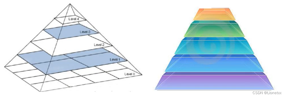
Image pyramid It is a kind of multi-scale expression in image , It is mainly used for image segmentation , It is an effective and simple structure to interpret images with multi-resolution . Simply speaking , Image pyramid is a collection of subgraphs with different resolutions of the same image ( Yes 800×800、480×640…)
Image pyramids were originally used for Machine vision and Image compression , The pyramid of an image is a series arranged in the shape of a pyramid The resolution gradually decreases 、 And From the same original picture Of Image set . It is obtained by step down sampling , Stop sampling until a certain termination condition is reached .
At the bottom of the pyramid is a high-resolution representation of the image to be processed , And at the top is a low resolution approximation . We compare layers of images to pyramids , The higher the level , The smaller the image , Lower resolution
The Gaussian pyramid fixes the zoom ratio , That is, if you are 800×800 Graph , Cannot zoom to 500×500
We are going to learn how to use , How to generate these image pyramids
There are two common types of image pyramids :
- The pyramid of Gauss (Gaussian pyramid): Used to go down / Downsampling ( Resolution decreases , The picture gets smaller , Go up ), Is the main image pyramid ;
- The pyramid of Laplace (Laplacian pyramid): It is used to reconstruct the upper unsampled image from the lower image of the pyramid , In digital image processing, that is, prediction residual , The image can be restored to the greatest extent , Use with Gaussian pyramid
The pyramid of Gauss (Gaussian pyramid)
The pyramid of Gauss It is through Gaussian smoothing and sub sampling ( Take a small piece out of a figure ) A series of gains Down sampling image
Down sampling
The principle is very simple : As shown in the figure below 
Original image resolution M*N ——> Resolution after image processing M/2 * N/2; That is, after each treatment , The result is the original 1/4( Even numbers are not required , It will automatically round )
Be careful : Down sampling ( Resolution decreases , In the above figure, it is shown as Direction up ) Information will be lost
The key API:cv2.pyrDown(src[, dst[, dstsize[, borderType]]])
among :
src: Pictures that need to be operateddst: Return value , Do not write , We can accept it with a parameterdstsize: Returns the size of the picture- The picture will become the original 1/4
#  The pyramid of Gauss  ——>  Down sampling

import cv2
import numpy as np

img = cv2.imread('./lena.png')

#  Resolution reduction operation : Down sampling
dst = cv2.pyrDown(img)

#  It can be changed many times
dst2 = cv2.pyrDown(dst)

#  Exhibition
cv2.imshow('img',img)
cv2.imshow('dst',dst)
cv2.imshow('dst2',dst2)

cv2.waitKey(0)
cv2.destroyAllWindows()
result :
In fact, the clarity has hardly changed , This is the power of image pyramid : Even rows and even columns are lost , however After Gaussian kernel convolution , It's equivalent to smoothing a pixel around , Therefore, there is little change
Sampling up
Up sampling is the opposite process of down sampling , Refers to the process of the picture from small to large 
- Double the image in each direction , New rows and columns with 0 fill
- Use the same kernel as before ( multiply 4) Convolute the enlarged image , Get an approximation ——> Suppose a group of four , It is equivalent to turning the place with value to three around 0 Fill in the position of **( Take the upper left corner for example , Is equivalent to 10 Divide into four , One copy 2.5; But because the overall value becomes smaller , The image will be dimmed , To solve this problem , Let's take 4, amount to “ Copy ” Four copies )**
The operation is the same as down sampling !
The key API:cv2.pyrUp(src[, dst[, dstsize[, borderType]]])
among :
src: Pictures that need to be operateddst: Return value , Do not write , We can accept it with a parameterdstsize: Returns the size of the picture- The picture will become the original 4 times
#  The pyramid of Gauss  ——>  Sampling up

import cv2
import numpy as np

img = cv2.imread('./Hello.jpeg')

#  Resolution reduction operation : Down sampling
dst = cv2.pyrUp(img)

#  It can be changed many times
# dst2 = cv2.pyrUp(dst)

#  Exhibition
cv2.imshow('img',img)
cv2.imshow('dst',dst)
# cv2.imshow('dst2',dst2)

cv2.waitKey(0)
cv2.destroyAllWindows()
result :
The pyramid of Laplace

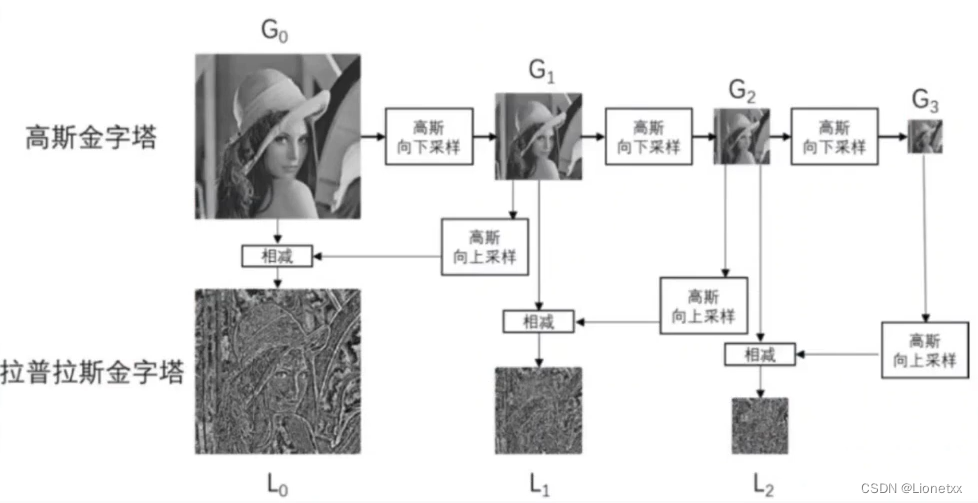
Laplace pyramid image = original image - Shangcai operation function ( Mining operation function ( original image ))
The image after downsampling is upsampled , Then make an error with the original image that has not been downsampled before to obtain the residual image ! Prepare information for restoring images !
in other words , The pyramid of Laplace It's universal Original image subtract An image that shrinks first and then enlarges ( The pyramid of Gauss ) A series of images of , The result of subtraction is the image of Laplace pyramid . What is retained is the residual !
Laplace pyramid is made up of Gauss pyramid , There are no special functions
#  The pyramid of Laplace
#  Original picture  -  Zoom in and out ( In this way, it can be changed back to the original size , Convenient to do bad )

import cv2
import numpy as np

img = cv2.imread('./lena.png')

#  Shrink first
temp = cv2.pyrDown(img)

#  Zoom in
dst = cv2.pyrUp(temp)

#  Original picture   and   The pyramid of Gauss   The difference is   The pyramid of Laplace
lap0 = img - dst

#  Exhibition
# cv2.imshow('img',img)
cv2.imshow('dst',dst)
cv2.imshow('lap0',lap0)

cv2.waitKey(0)
cv2.destroyAllWindows()
result :
Image histogram
The basic concept of image histogram
In statistics , Histogram is a graphical representation of the distribution of data , It's a two-dimensional statistical chart
Image histogram Is a histogram used to represent the brightness distribution in a digital image , Plotted The number of pixels per luminance value in the image .
By observing the histogram, you can know how to adjust the histogram of brightness distribution . In this histogram , The left side of the abscissa is solid black 、 Darker areas , and The right side is brighter 、 Pure white areas .
therefore , The data of the image histogram of a darker picture is mostly concentrated in the left and middle parts , And the whole is bright , Images with only a few shadows are the opposite
- Abscissa : Of each pixel in the image Gray scale ( Gray value 0-255 Every number is a gray level )
- Ordinate : With this gray level Number of pixels

We can see from the image histogram : There are many dark or bright points in this image ( There are many pixels with these gray levels ), On the contrary, there are fewer points of light dark balance **( There are fewer pixels with these gray levels )**
After understanding it, we can independently analyze the following three pictures ( Too lazy to write. …)

Take up a :
There is one 3×3 Pictures of the , among
- Gray level of pixels Express ——> What numbers are there in the picture
- The number of pixels with this gray level Express ——> This number appears several times in the picture

Draw the histogram above , There are many kinds of histograms . such as :
Broken line diagram :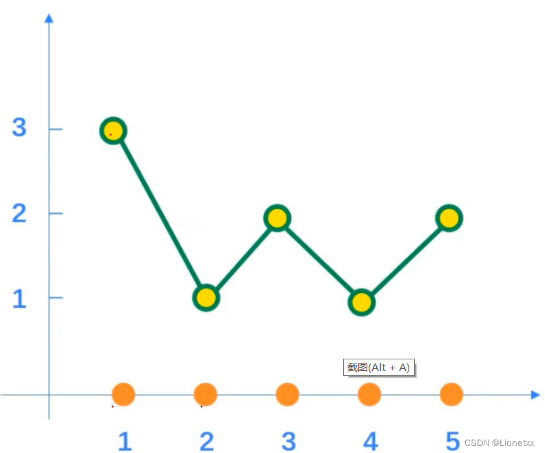
Histogram :
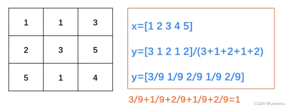
Normalized graph :
- Abscissa : Of each pixel in the image Gray scale ( The pixel value appearing in the image )
- Ordinate : This gray level appears probability ( The number of times each pixel value appears in the image / Number of pixel values )
Histogram terminology
dims: The number of features to be counted in the histogram , That is, the items that need to be counted . Such as dims = 1, It means that we only use the statistical gray valuebins: Between each cell in the histogram ( Each feature space sub segment ) Number of , Operate more often
range: We count the range of gray values , It's usually 0-255
in general : Histogram is a graph drawn by the number of times various gray levels appear in the image
Use OpenCV Statistical histogram
The key API:cv2.calcHist(images, channels, mask, histSize, ranges[, hist[, accumulate]])
images: original image ( It can not be black and white ), AddsIt means that histogram statistics can be carried out on multiple pictures at the same time ——> Brackets should be added here , The representation is a collection of imageschannels: Designated channel , You need brackets "[ ]" Cover up- If the input image is a grayscale image , Then there is only one channel , be [ ] Write in 0:
[0] - Color images can be
[ 0 ], [ 1 ], [ 2 ], They correspond to each other B,G,R
- If the input image is a grayscale image , Then there is only one channel , be [ ] Write in 0:
mask: Mask image- Count the histogram of the whole image : Set to
None - Statistics of the histogram of an area of the image : Mask image required
- Count the histogram of the whole image : Set to
histSize:BINS( The column in the histogram ) The number of- It needs to be enclosed in brackets , Such as
[256]( Because from 0 Start , So there is 256 A digital )
- It needs to be enclosed in brackets , Such as
ranges: Pixel value range , for example[0,255]accumulate: Cumulative identification- The default value is
False( Generally, we only operate on one graph ) - If it is set to
True, be The histogram will not be cleared at the beginning of allocation - This parameter allows the calculation of a single histogram from multiple objects , Or to update histograms in real time
- Cumulative results of multiple histograms , Used to calculate histogram for a set of images
- The default value is
- This function will return the data of histogram , It can be used directly
plt.plot( Return value )Draw !
# OpenCV Statistical histogram

import cv2
import numpy as np

img = cv2.imread('./lena.png')

hist = cv2.calcHist([img],[0],None,[256],[0,255])
print(hist)
result :
From top to bottom are Gray scale 0、1、2......
Use OpenCV Draw histogram
#  Draw histogram
#  Use Opencv The statistical method of

import cv2
import numpy as np
import matplotlib.pyplot as plt

img = cv2.imread('./lena.png')

#  Statistical histogram data , Don't do grayscale pictures anymore ( Parameters channels The channel can be counted )
hist_B = cv2.calcHist([img],[0],None,[256],[0,255])
hist_G = cv2.calcHist([img],[1],None,[256],[0,255])
hist_R = cv2.calcHist([img],[2],None,[256],[0,255])

#  Three data are obtained above , We draw three pictures correspondingly , Mark different colors
plt.plot(hist_B,color = 'b',label = 'Blue') #  No more hist(), Because what is returned is histogram data
plt.plot(hist_G,color = 'g',label = 'Green')
plt.plot(hist_R,color = 'r',label = 'Red')
plt.legend() #  Put instructions on the shaft
#  Exhibition ( Add it or not )
plt.show()
result :
The corresponding horizontal axis is converted from gray value ( We don't give the value of the horizontal axis ,matplotlib Automatically indexed , amount to cv2.cvtColor(img,cv2.COLOR_GRAY2BRR))
We can find out : The whole picture is red ( Red low frequency is less , There are many in the high-frequency region ), Blue is on the low side ( Only a little on the hat ), Green is less in the high frequency region ( There is almost no green in the whole picture )

Use the histogram of the mask
If you are only interested in a certain part of the picture ( For example, the face in the image 、 hand …), You can use it A mask To operate , Select roi Area , Use for this area cv2.calcHist(mask) Histogram calculation
- A mask
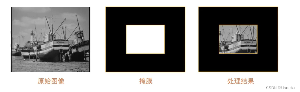
Characteristics of mask : The area you want to display is pure white , Other areas you don't want it to display are pure black - How to generate a mask
- Mr. Cheng is the same size as the original picture (
img.shape) All black pictures of :mask = np.zeros(image.shape,np.uint8) - Set the desired region as 255:
mask[100:200,200:300] = 355
- Mr. Cheng is the same size as the original picture (
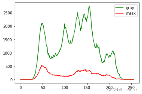
#  Use the histogram of the mask

import cv2
import numpy as np
import matplotlib.pyplot as plt

img = cv2.imread('./lena.png')

#  Turn into a black-and-white picture
gray = cv2.cvtColor(img,cv2.COLOR_BGR2GRAY)

#  Generate mask image
mask = np.zeros(gray.shape,np.uint8) #  Generate an all black graph with the same size as the original one  uint8:8 Bits are all used to represent numbers

#  Set the area where you want to count the histogram (roi)
mask[200:400,200:400] = 255

#  Statistical histogram data  ——>  Compare the original image with the data after mask operation
hist_gray = cv2.calcHist([gray],[0],None,[256],[0,255])
hist_mask = cv2.calcHist([gray],[0],mask,[256],[0,255])

#  Use matplotlib Draw a histogram
plt.plot(hist_gray,label = 'gray',color = 'g')
plt.plot(hist_mask,label = 'mask',color = 'r')
plt.legend()
plt.show()

##---------------------------------------------------------------------------------------------
#  We want to see the effect of the mask in the picture in advance
cv2.imshow('gray',gray)
cv2.imshow('mask',mask)

# gray  and  gray  And the result of the operation is itself  mask The role of : First do and operation , The results will be compared with mask Do with the operation
#  Characteristics of and operation : Two numbers “ And ”,0 And any number is 0,255 He Fei 0 Of “ And ” are 0 In itself ( Original picture )
cv2.imshow('gray&mask',cv2.bitwise_and(gray,gray,mask = mask))
##---------------------------------------------------------------------------------------------

#  Exit conditions
cv2.waitKey(0)
cv2.destroyAllWindows()
result :
边栏推荐
- 容错、熔断的使用与扩展
- Overview of MES system equipment management (medium)
- [I also want to brush through leetcode] 468. Verify the IP address
- Buckle exercise - 32 divided into k equal subsets
- Force deduction exercise - 26 split array into continuous subsequences
- TypeNameExtractor could not be found
- [rust] Why do I suggest you learn rust | a preliminary study of rust
- An analysis of the CPU surge of an RFID tag management system in.Net
- One week's wonderful content sharing (issue 13)
- Aruba learning notes 04 Web UI -- Introduction to configuration panel
猜你喜欢

In kuborad graphical interface, operate kubernetes cluster to realize master-slave replication in MySQL

Zhihuihuayun | cluster log dynamic collection scheme

Convergence rules for 4 * 4 image weights
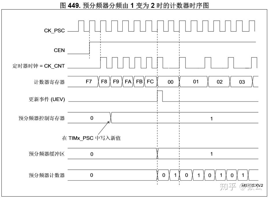
What is prescaler in STM32

Miss waiting for a year! Baidu super chain digital publishing service is limited to 50% discount
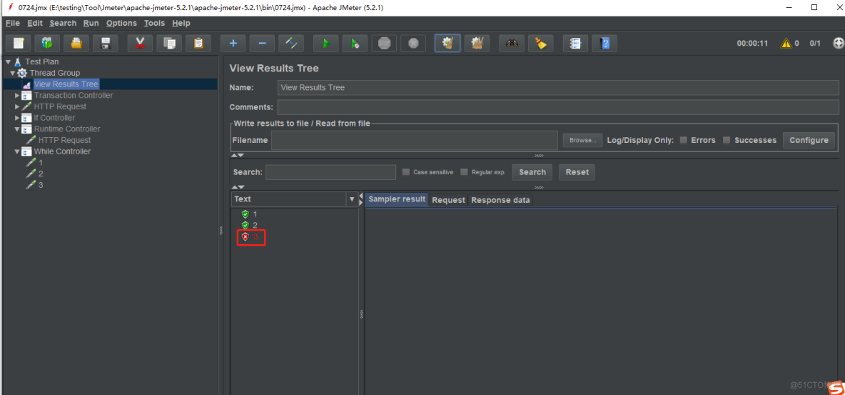
JMeter while controller

Dynamic memory management

One week's wonderful content sharing (issue 13)

QT notes - qtablewidget table spanning tree, qtreewidget tree node generates table content

【C和指针第14章】预处理器
随机推荐
Most after analyze table in PostgreSQL_ common_ Why is the elems field not filled in?
Calculate the distance between the longitude and latitude of two coordinates (5 ways)
Miss waiting for a year! Baidu super chain digital publishing service is limited to 50% discount
AcWing 92. 递归实现指数型枚举
动态内存管理
Buckle practice - 25 non overlapping intervals
如何在IM系统中实现抢红包功能?
Online XML to CSV tool
L1-059 ring stupid bell
L1-059 敲笨钟
MySQL advanced (XVII) cannot connect to database server problem analysis
字符串匹配的KMP
Oceanbase Database Setup Test
TypeNameExtractor could not be found
CCF 1-2 question answering record (1)
理解数据的存与取
What is prescaler in STM32
Zhihuihuayun | cluster log dynamic collection scheme
In kuborad graphical interface, operate kubernetes cluster to realize master-slave replication in MySQL
try...finally总结