Deriving Kalman filter from probability theory

In this paper, the scalar and vector Kalman filter is derived from some properties of joint normal distribution . Some of the following properties have been named for convenience , Not necessarily a formal academic name .
ps: There are several properties I can't prove , Welcome to correct .
The official certificate has not been written yet .

Description of formulas and symbols

Discrete systems
$$\begin{array}{rl}& x(k)=Ax(k-1)+Bu(k-1)+v(k-1)\\ & y(k)=Cx(k)+W(k)\end{array}$$
among $V,W$ Is the covariance matrix of zero mean Gaussian white noise .
The recurrence formula of Kalman filter is as follows
x ^ ( k ∣ k − 1 ) = A x ^ ( k − 1 ) + B u ( k − 1 ) x ^ ( k ) = x ^ ( k ∣ k − 1 ) + K ( k ) [ y ( k ) − C x ^ ( k ∣ k − 1 ) ] P ( k ∣ k − 1 ) = A P ( k − 1 ) A T + V P ( k ) = [ I − K ( k ) C ] P ( k ∣ k − 1 ) K ( k ) = P ( k ∣ k − 1 ) C T [ C P ( k ∣ k − 1 ) C T + W ] − 1 \begin{aligned} & \hat{x}(k|k-1)=A\hat{x}(k-1)+Bu(k-1) \\ & \hat{x}(k)=\hat{x}(k|k-1)+K(k)[y(k)-C\hat{x}(k|k-1)] \\ & P(k|k-1)=AP(k-1)A^{\text{T}}+V \\ & P(k)=[I-K(k)C]P(k|k-1) \\ & K(k)=P(k|k-1)C^{\text{T}}[CP(k|k-1)C^{\text{T}}+W]^{-1} \\ \end{aligned} ​x^(k∣k−1)=Ax^(k−1)+Bu(k−1)x^(k)=x^(k∣k−1)+K(k)[y(k)−Cx^(k∣k−1)]P(k∣k−1)=AP(k−1)AT+VP(k)=[I−K(k)C]P(k∣k−1)K(k)=P(k∣k−1)CT[CP(k∣k−1)CT+W]−1​

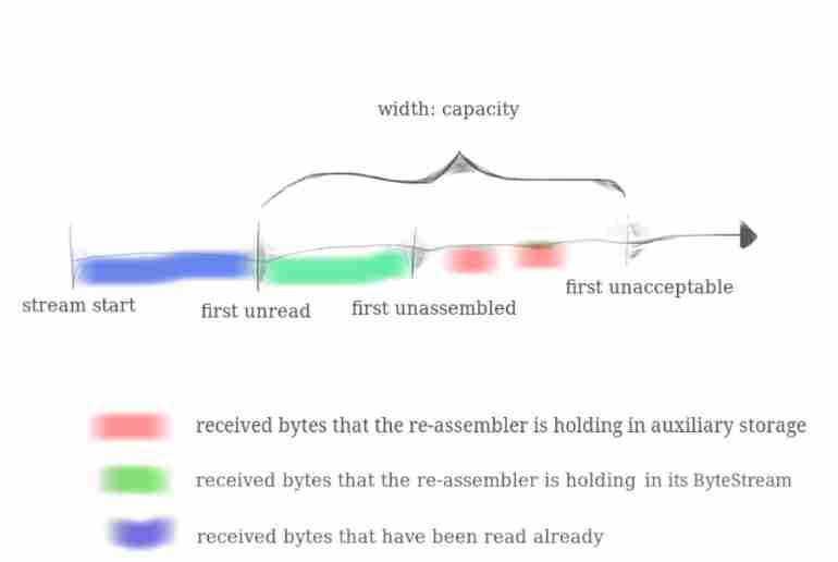
• $\mathbf{Y}(k)=[y(0),y(1),\cdots ,y(k)]$ Before presentation $k$ Observation data at a time
• $\hat{x}(k)=\text{E}[x(k)|Y(k)]$ According to the previous $k$ Prediction of observed data at a time $x(k)$
• $\hat{x}(k|k-1)$ According to the previous $k-1$ Prediction of observed data at a time $x(k)$
• $P(k)$ Indicates the estimation error
• $P(k|k-1)$ Represents the prediction error

Several properties and partial proofs

Bayesian least mean square error estimator (Bmse)
Observed $x$ after $\theta$ The least mean square error estimator of $\hat{\theta }$ by
$$\hat{\theta }=\text{E}(\theta |x)$$
The main idea of proof is to find $\hat{\theta }$ Minimize the minimum mean square error . prove ：
$$\begin{array}{rl}\text{Bmse}(\hat{\theta })& =\text{E}[(\theta -\hat{\theta }{)}^2]\\ & =\iint (\theta -\hat{\theta }{)}^{2}p(x,\theta )\text{d}x\text{d}\theta \\ & =\int \left[\int (\theta -\hat{\theta }{)}^{2}p(\theta |x)\text{d}\theta \right]p(x)\text{d}x\\ J& =\int (\theta -\hat{\theta }{)}^{2}p(\theta |x)\text{d}\theta \\ \frac{\partial J}{\partial \hat{\theta }}& =-2\int \theta p(\theta |x)\text{d}\theta +2\hat{\theta }\int p(\theta |x)\text{d}\theta =0\\ \hat{\theta }& =\frac{2\int \theta p(\theta |x)\text{d}\theta }{2\int p(\theta |x)\text{d}\theta }=\text{E}(\theta |x)\end{array}$$
Zero mean application theorem ( Scalar form )
set up $x$ and $y$ Is a random variable with joint normal distribution , be
$$\begin{array}{rl}& \text{E}(y|x)=\text{E}y+\frac{\text{Cov}(x,y)}{\text{D}x}(x-\text{E}x)\\ & \text{D}(y|x)=\text{D}y-\frac{{\text{Cov}}^2(x,y)}{\text{D}x}\end{array}$$
The two forms can be written separately
$$\begin{array}{rl}& \frac{\hat{y}-\text{E}y}{\sqrt{\text{D}y}}=\rho \frac{x-\text{E}x}{\sqrt{\text{D}x}}\\ & \text{D}(y|x)=\text{D}y(1-{\rho }^2)\end{array}$$
prove ：
$$\begin{array}{rl}\hat{y}& =ax+b\\ J& =\text{E}(y-\hat{y}{)}^2\\ & =\text{E}[y^2-2y(ax+b)+(ax+b{)}^2]\\ & =y^2-2\text{E}xy\cdot a-2\text{E}y\cdot b+\text{E}{x}^2\cdot a^2+2\text{E}x\cdot ab+b^2\\ \text{d}J& =(-2\text{E}xy+2\text{E}{x}^2+2b\text{E}x)\text{d}a+(-2\text{E}y+2a\text{E}x+2b)\text{d}b\\ \frac{\partial J}{\partial a}& =-2\text{E}xy+2\text{E}{x}^2+2b\text{E}x=0\\ \frac{\partial J}{\partial b}& =-2\text{E}y+2a\text{E}x+2b=0\\ b& =\frac{\text{E}xy-\text{E}{x}^2}{\text{E}x}\\ a& =\frac{\text{E}y-b}{\text{E}x}=\frac{\text{E}x\text{E}y-\text{E}xy+\text{E}{x}^2}{(\text{E}x{)}^2}\\ \hat{y}& =ax+b=\end{array}$$
The theorem is only valid for random variables that satisfy linear relations including normal distribution ( It is not clear where the linearity is satisfied ). for example , For two joint uniform distributions
$$\begin{array}{rl}& f(x,y)=2,0<x<1,0<y<x\\ & f(x,y)=3,0<x<1,x^2<y<\sqrt{x}\end{array}$$
The first was established , The second one does not hold because of the existence of nonlinearity , in other words $y$ In the data $x$ The linear Bayesian estimator under is not the best estimator , The two are
$$\begin{array}{rl}& \hat{y}=\text{E}y+\frac{\text{Cov}(x,y)}{\text{D}x}(x-\text{E}x)=\frac{133x+9}{153}\\ & \hat{y}=\text{E}(y|x)=\frac{\sqrt{x}+x^2}{2}\end{array}$$
Zero mean application theorem ( Vector form )
$\mathbf{x}$ and $\mathbf{y}$ Is a random vector of joint normal distribution ,$\mathbf{x}$ yes m×1,$\mathbf{y}$ yes n×1, Block covariance matrix
$$\mathbf{C}=\left[\begin{array}{cc}{\mathbf{C}}_{xx}& {\mathbf{C}}_{xy}\\ {\mathbf{C}}_{yx}& {\mathbf{C}}_{yy}\end{array}\right]$$
be
$$\text{E}(\mathbf{y}|\mathbf{x})=\text{E}(\mathbf{y})+{\mathbf{C}}_{yx}{\mathbf{C}}_{xx}^{-1}(\mathbf{x}-\text{E}(\mathbf{x}))$$
among $C_{xy}$ Express $\text{Cov}(x,y)$. prove ：
$$\begin{array}{rl}\hat{y}& =Ax+b\\ J& =\text{E}(y-\hat{y}{)}^{\top }(y-\hat{y})\\ & =\text{E}(y^{\top }y-{\hat{y}}^{\top }y-y^{\top }\hat{y}+{\hat{y}}^{\top }\hat{y})\\ \text{d}J& =\text{dE}(-{\hat{y}}^{\top }y-y^{\top }\hat{y}+{\hat{y}}^{\top }\hat{y})\\ & =\text{dE}[\text{tr}(-{\hat{y}}^{\top }y-y^{\top }\hat{y}+{\hat{y}}^{\top }\hat{y})]\\ & =\cdots \\ A& =C_{xx}^{-1}{C}_{xy}\\ b& =\text{E}y-A\text{E}x\\ \hat{y}& =C_{xx}^{-1}{C}_{xy}x+\text{E}y-C_{xx}^{-1}{C}_{xy}\text{E}x\\ & =\text{E}y+C_{xx}^{-1}{C}_{xy}(x-\text{E}x)\end{array}$$
Projection theorem ( Orthogonal principle )

   When using the linear combination of data samples to estimate a random variable , When the error between the estimated value and the true value is orthogonal to each data sample , This estimate is the best estimate , Data samples $x$ And the best estimator $\hat{y}$ Satisfy
$$\text{E}[(y-\hat{y}{)}^{\top }x(n)]=0n=0,1,\cdots ,N-1$$
   Random variables with zero mean satisfy the properties in inner product space . Define the length of the variable $||x||=\sqrt{\text{E}{x}^2}$, Variable $x$ and $y$ Inner product $(x,y)$ Defined as $\text{E}(xy)$, The angle between two variables is defined as the correlation coefficient $\rho$. When $\text{E}(xy)=0$ Time variable $x$ and $y$ orthogonal .
   When the mean value is not zero , Define the length of the variable $||x||=\sqrt{\text{D}x}$, Variable $x$ and $y$ Inner product $(x,y)$ Defined as $\text{Cov}(xy)$, The angle between two variables is defined as the correlation coefficient $\rho$. The case that the mean value is not zero is my own guess , A lot of information is not detailed , But the derivation of Kalman filter is all non-zero mean .
   take $x$ and $y$ Corresponding to the form of data , namely $x(0)$ yes $x$,$x(1)$ yes $y$,$\hat{x}(1|0)$ yes $\hat{y}$, obtain
$$\text{E}[(x(1)-\hat{x}(1|0){)}^{\top }x(0)]=0$$
among
$$\tilde{x}(k|k-1)=x(k)-\hat{x}(k|k-1)$$
It is called new interest (innovation), With old data $x(0)$ orthogonal .
   Scalar formal proof ：
$$\begin{array}{rl}\text{E}[x(\hat{y}-y)]& =\text{E}[x\text{E}y+\frac{\text{Cov}(x,y)}{\text{D}x}(x^2-x\text{E}x)-xy]\\ & =\text{E}x\text{E}y+\frac{\text{Cov}(x,y)}{\text{D}x}(\text{E}{x}^2-(\text{E}x{)}^2)-\text{E}xy\\ & =\text{Cov}(x,y)+\text{E}x\text{E}y-\text{E}xy=0\end{array}$$
   Vector form proof ：
$$\begin{array}{rl}\text{E}[x^{\top }(\hat{y}-y)]& =\text{E}[x^{\top }\text{E}y+x^{\top }{C}_{xx}^{-1}{C}_{xy}(x-\text{E}x)]\\ & =\cdots \\ & =0\end{array}$$
   because $\text{E}(y-\hat{y})=0$, Therefore, the orthogonal condition also holds when the mean value is non-zero . Another formula of projection theorem can be obtained from graph
$$\text{E}[(y-\hat{y})\hat{y}]=0$$
prove ：
$$\begin{array}{rl}& \text{E}[\hat{y}(\hat{y}-y)]\\ =& \text{E}[(\text{E}y+kx-k\text{E}x)(\text{E}y+kx-k\text{E}x-y)]\\ =& (\text{E}y{)}^2+k\text{E}x\text{E}y-k\text{E}x\text{E}y-(\text{E}y{)}^2\\ & +k\text{E}x\text{E}y+k^{2}E{x}^2-k^2(\text{E}x{)}^2-k\text{E}xy\\ & -k\text{E}x\text{E}y-k^2(\text{E}x{)}^2+k^2(\text{E}x{)}^2+k\text{E}x\text{E}y\\ =& k^2\text{D}x-k\text{Cov}(x,y)\\ =& \frac{[\text{Cov}(x,y){]}^2}{[\text{D}x{]}^2}\text{D}x-\frac{\text{Cov}(x,y)}{\text{D}x}\text{Cov}(x,y)\\ =& 0\end{array}$$
Expected additivity
$\text{E}[y_1+y_2|x]=\text{E}[y_1|x]+\text{E}[y_2|x]$
Independent conditional additivity
if $x_1$ and $x_2$ Independent , be
$$\text{E}[y|x_1,x_2]=\text{E}[y|x_1]+\text{E}[y|x_2]-\text{E}y$$
prove ：
Make $x=[x_1^{\top },x_2^{\top }{]}^{\top }$, be
$$\begin{array}{rl}{C}_{xx}^{-1}& ={\left[\begin{array}{cc}{C}_{x_1{x}_1}& C_{x_1{x}_2}\\ C_{x_2{x}_1}& C_{x_2{x}_2}\end{array}\right]}^{-1}=\left[\begin{array}{cc}{C}_{x_1{x}_1}^{-1}& O\\ O& C_{x_2{x}_2}^{-1}\end{array}\right]\\ C_{yx}& =\left[\begin{array}{cc}{C}_{y{x}_1}& C_{y{x}_2}\end{array}\right]\\ \text{E}(y|x)& =\text{E}y+C_{yx}{C}_{xx}^{-1}(x-\text{E}x)\\ & =\text{E}y+\left[\begin{array}{cc}{C}_{y{x}_1}& C_{y{x}_2}\end{array}\right]\left[\begin{array}{cc}{C}_{x_1{x}_1}^{-1}& O\\ O& C_{x_2{x}_2}^{-1}\end{array}\right]\left[\begin{array}{c}{x}_1-\text{E}{x}_1\\ x_2-\text{E}{x}_2\end{array}\right]\\ & =\text{E}[y|x_1]+\text{E}[y|x_2]-\text{E}y\end{array}$$
Dependent conditional additivity ( Innovation theorem )
if $x_1$ and $x_2$ Not independent , According to the projection theorem $x_2$ And $x_1$ Independent components ${\tilde{x}}_2$, Satisfy
$$\text{E}[y|x_1,x_2]=\text{E}[y|x_1,{\tilde{x}}_2]=\text{E}[y|x_1]+\text{E}[y|{\tilde{x}}_2]-\text{E}y$$
among ${\tilde{x}}_2=x_2-{\hat{x}}_2=x_2-\text{E}(x_1|x_2)$, By the projection theorem ,$x_1$ And ${\tilde{x}}_2$ Independent ,${\tilde{x}}_2$ It is called new interest .
prove ( Each of the following formulas is to find the part first and then the whole , For ease of understanding, you can look from bottom to top )：
$$\begin{array}{rl}\text{E}(y|x_1,x_2)& =\text{E}y+\frac{\left[\begin{array}{cc}{C}_{y{x}_1}& C_{y{x}_2}\end{array}\right]}{\text{D}{x}_1\text{D}{x}_2-C_{x_1{x}_2}^2}\left[\begin{array}{cc}\text{D}{x}_2& -C_{x_1{x}_2}\\ -C_{x_1{x}_2}& \text{D}{x}_1\end{array}\right]\left[\begin{array}{c}{x}_1-\text{E}{x}_1\\ x_2-\text{E}{x}_2\end{array}\right]\\ \text{Cov}(y,{\hat{x}}_2)& =\text{E}[y\left(\text{E}{x}_2+\frac{\text{Cov}(x_2,x_1)}{\text{D}{x}_1}(x_1-\text{E}{x}_1)\right)]-\text{E}y\text{E}{\hat{x}}_2\\ & =\text{E}y\text{E}{x}_2+\frac{\text{Cov}(x_2,x_1)}{\text{D}{x}_1}(\text{E}{x}_{1}y-\text{E}{x}_1\text{E}y)-\text{E}y\text{E}{x}_2\\ & =\frac{C_{x_1{x}_2}{C}_{y{x}_1}}{\text{D}{x}_1}\\ \text{Cov}(x_2,{\hat{x}}_2)& =\text{E}{x}_2{\hat{x}}_2-\text{E}{x}_2\text{E}{\hat{x}}_2\\ & =\text{E}[x_2(\text{E}{x}_2+\frac{\text{Cov}(x_2,x_1)}{\text{D}{x}_1}(x_1-\text{E}{x}_1))]-(\text{E}{x}_2{)}^2\\ & =\frac{C_{x_1{x}_2}^2}{\text{D}{x}_1}\\ \text{D}{\hat{x}}_2& =\text{D}(\text{E}{x}_2+\frac{\text{Cov}(x_2,x_1)}{\text{D}{x}_1}(x_1-\text{E}{x}_1))\\ & =\frac{C_{x_1{x}_2}^2}{(\text{D}{x}_1{)}^2}\text{D}{x}_1=\frac{C_{x_1{x}_2}^2}{\text{D}{x}_1}\\ \text{D}{\tilde{x}}_2& =\text{D}{x}_2+\text{D}{\hat{x}}_2-2\text{Cov}(x_2,{\hat{x}}_2)\\ & =\text{D}{x}_2-\frac{C_{x_1{x}_2}^2}{\text{D}{x}_1}\\ \text{E}[y|x_1]+\text{E}[y|{\tilde{x}}_2]-\text{E}y& =\text{E}y+\frac{C_{x_{1}y}}{\text{D}{x}_1}(x_1-\text{E}{x}_1)+\frac{\text{Cov}(y,{\tilde{x}}_2)}{\text{D}{\tilde{x}}_2}({\tilde{x}}_2-\text{E}{\tilde{x}}_2)\\ & =\cdots +\frac{\text{Cov}(y,x_2)-\text{Cov}(y,{\hat{x}}_2)}{\text{D}{\tilde{x}}_2}(x_2-{\hat{x}}_2)\\ & =\cdots +\frac{C_{y{x}_2}-\frac{C_{x_1{x}_2}{C}_{y{x}_1}}{\text{D}{x}_1}}{\text{D}{x}_2-\frac{C_{x_1{x}_2}^2}{\text{D}{x}_1}}(x_2-{\text{E}}_2-\frac{\text{Cov}(x_2,x_1)}{\text{D}{x}_1}(x_1-{\text{E}}_1))\\ & =\cdots +\frac{C_{y{x}_2}\text{D}{x}_1-C_{x_1{x}_2}{C}_{y{x}_1}}{\text{D}{x}_1\text{D}{x}_2-C_{x_1{x}_2}^2}(x_2-{\text{E}}_2-\frac{C_{x_1{x}_2}}{\text{D}{x}_1}(x_1-{\text{E}}_1))\\ & =\text{E}y+A(x_1-\text{E}{x}_1)+B(x_2-{\text{E}}_2)\end{array}$$
among
$$\begin{array}{rl}B& =\frac{C_{y{x}_2}\text{D}{x}_1-C_{x_1{x}_2}{C}_{y{x}_1}}{\text{D}{x}_1\text{D}{x}_2-C_{x_1{x}_2}^2}\\ A& =\frac{C_{x_{1}y}}{\text{D}{x}_1}-B\frac{C_{x_1{x}_2}}{\text{D}{x}_1}\end{array}$$
In another equation $\text{E}(y|x_1,x_2)$ in ,
$$\begin{array}{rl}A& =\frac{C_{y{x}_1}\text{D}{x}_2-C_{y{x}_2}{C}_{x_1{x}_2}}{\text{D}{x}_1\text{D}{x}_2-C_{x_1{x}_2}^2}\\ B& =\frac{C_{y{x}_2}\text{D}{x}_1-C_{y{x}_1}{C}_{x_1{x}_2}}{\text{D}{x}_1\text{D}{x}_2-C_{x_1{x}_2}^2}\end{array}$$
The two expressions are equal .

DC level in Gaussian white noise

This example can be used as a cushion , It is helpful to understand the source of each formula of Kalman filter , such as $x(k)$ and $x(k-1)$ Why should there be a $\hat{x}(k|k-1)$ etc. . Consider the model
$$x(k)=A+w(k)$$
among $A$ Is the parameter to be estimated ,$w(k)$ Yes, the mean is 0、 The variance of ${\sigma }^2$ The Gaussian white noise of ,$x(k)$ It's observation . You can get $\hat{x}(0)=x(0)$, And then according to $x(0)$ and $x(1)$ forecast $k=1$ The value of the moment $\text{E}[x(1)|x(1),x(0)]$ when , Conditional additivity of the joint normal distribution is required , But because of $x(1)$ and $x(0)$ Not independent , You need to use the projection theorem to calculate two independent variables $x(0)$ And $\tilde{x}(1|0)$, And then calculate $\hat{x}(1)$, namely
$$\begin{array}{rl}\hat{x}(1)& =\text{E}[x(1)|x(1),x(0)]\\ & =\text{E}[x(1)|x(0),\tilde{x}(1|0)]\\ & =\text{E}[x(1)|x(0)]+\text{E}[x(1)|\tilde{x}(1|0)]-\text{E}x(1)\end{array}$$
among $\text{E}[x(1)|x(0)]=\hat{x}(1|0)$,
$$\begin{array}{rl}\hat{x}(1|0)& =\text{E}x(1)+\frac{\text{Cov}(x(1),x(0))}{\text{D}x(0)}(x(0)-\text{E}x(0))\\ & =A+\frac{\text{E}(A+w(1))(A+w(0))-\text{E}(A+w(1))\text{E}(A+w(0))}{\text{E}(A+w(1){)}^2-[\text{E}(A+w(1)){]}^2}(x(0)-A)\\ & =A\end{array}$$
In this case, there appears $\hat{x}(k|k-1)$, And another unknown formula $\text{E}[x(1)|\tilde{x}(1|0)]$. Apply the theorem from zero mean ,
$$\text{E}[x(1)|\tilde{x}(1|0)]=\text{E}x(0)+\frac{\text{Cov}(x(1),\tilde{x}(1|0))}{\text{D}\tilde{x}(1|0)}(\tilde{x}(1|0)-\text{E}\tilde{x}(1|0))$$
among
$$\begin{array}{rl}\tilde{x}(1|0)& =x(1)-\hat{x}(1|0)\\ \text{E}\tilde{x}(1|0)& =\text{E}(x-\hat{x})=0\\ \text{D}\tilde{x}(1|0)& =\text{E}(x(1)-\hat{x}(1|0){)}^2\\ & =\text{E}(A+w(1){)}^2\\ & =a^{2}P(0)+{\sigma }^2\\ & =P(1|0)\end{array}$$

Kalman filter is formally derived

Scalar form
$$\begin{array}{rl}\hat{x}(k|k-1)& =\text{E}[x(k)|Y(k-1)]\\ & =\text{E}[ax(k-1)+bu(k-1)+v(k-1)|Y(k-1)]\\ & =a\text{E}[x(k-1)|Y(k-1)]+b\text{E}[u(k-1)|Y(k-1)]+\text{E}[v(k-1)|Y(k-1)]\\ & =a\hat{x}(k-1)+bu(k-1)\\ \tilde{x}(k|k-1)& =x(k)-\hat{x}(k|k-1)\\ & =(ax(k-1)+bu(k-1)+v(k-1))-(a\hat{x}(k-1)+bu(k-1))\\ & =a\tilde{x}(k-1)+v(k-1)\end{array}\text{\hspace{1em}(1)}$$
It is known that $\hat{x}(k)=\text{E}[x(k)|Y(k)]$, And because $\tilde{x}(k-1)$ contain $x(k)$,$x(k)$ Contain, $y(k)$, So the dataset $Y(k)$ Equivalent to data set $Y(k-1)$、$\tilde{x}(k|k-1)$, So by conditional additivity ,
$$\begin{array}{rl}\hat{x}(k)& =\text{E}[x(k)|Y(k-1),\tilde{x}(k-1)]\\ & =\text{E}[x(k)|Y(k-1)]+\text{E}[x(k)|\tilde{x}(k|k-1)]-\text{E}x(k)\\ & =\hat{x}(k|k-1)+\text{E}[x(k)|\tilde{x}(k|k-1)]-\text{E}x(k)\end{array}$$
Apply the theorem from zero mean ,
$$\text{E}[x(k)|\tilde{x}(k|k-1)]=\text{E}x(k)+\frac{\text{Cov}(x(k),\tilde{x}(k|k-1))}{\text{D}\tilde{x}(k|k-1)}(\tilde{x}(k|k-1)-\text{E}\tilde{x}(k|k-1))$$
among
$$\begin{array}{rl}\text{E}\tilde{x}(k|k-1)& =\text{E}(x-\hat{x})=0\\ \text{D}\tilde{x}(k|k-1)& =\text{E}(a\tilde{x}(k-1)+v(k-1){)}^2\\ & =a^{2}P(k-1)+V\\ & =P(k|k-1)\end{array}\text{\hspace{1em}(3)}$$
Make
$$M(k)=\frac{\text{Cov}(x(k),\tilde{x}(k|k-1))}{\text{D}\tilde{x}(k|k-1)}$$
be
$$\begin{array}{rl}\text{E}[x(k)|\tilde{x}(k|k-1)]& =\text{E}x(k)+M(k)(x(k)-\hat{x}(k|k-1))\\ \hat{x}(k)& =\text{E}[x(k)|Y(k-1),\tilde{x}(k-1)]\\ & =\text{E}[x(k)|Y(k-1)]+\text{E}[x(k)|\tilde{x}(k|k-1)]-\text{E}x(k)\\ & =\hat{x}(k|k-1)+M(k)(x(k)-\hat{x}(k|k-1))\end{array}$$
By the projection theorem $\text{E}[\hat{x}(x-\hat{x})]=0$ Calculation $M(k)$,
$$\begin{array}{rl}M(k)& =\frac{\text{Cov}(x(k),\tilde{x}(k|k-1))}{\text{D}\tilde{x}(k|k-1)}\\ & =\frac{\text{E}[x(k)(x(k)-\hat{x}(k|k-1))]-\text{E}x(k)\text{E}\tilde{x}(k|k-1)}{P(k|k-1)}\\ & =\frac{\text{E}[(x(k)-\hat{x}(k|k-1))(x(k)-\hat{x}(k|k-1))]}{P(k|k-1)}\end{array}$$
5 The equations are ,
(1) Prediction equation
(2) Correct the equation
(3) Minimum prediction mean square error
Vector form
$$\begin{array}{rl}\hat{x}(k|k-1)& =\text{E}[x(k)|Y(k-1)]\\ & =\text{E}[Ax(k-1)+Bu(k-1)+v(k-1)|Y(k-1)]\\ & =A\text{E}[x(k-1)|Y(k-1)]+B\text{E}[u(k-1)|Y(k-1)]+\text{E}[v(k-1)|Y(k-1)]\\ & =A\hat{x}(k-1)+Bu(k-1)\end{array}$$

Reference resources

• Sunzengqi . Computer control theory and application [M]. tsinghua university press , 2008.
• StevenM.Kay, Luopengfei . Fundamentals of statistical signal processing [M]. Electronic industry press , 2014.
• Zhaoshujie , Jian-xun zhao . Signal detection and estimation theory [M]. Electronic industry press , 2013.
• The derivation process of Kalman filter is explained in detail