Influence of air resistance on the trajectory of table tennis

Python Wechat ordering applet course video

https://edu.csdn.net/course/detail/36074

Python Actual quantitative transaction financial management system

https://edu.csdn.net/course/detail/35475 Catalog

• Technical background
• Simulation of air resistance
• The effect of adding a rotating arc circle
• Chopping curve
• Summary
• Copyright notice

---

Back to the top # Technical background

Table tennis is a national sport , It has not only collected many medals for China in the Olympic Games and many other sports venues , It is also popular among the people . stay Last blog It mainly describes the application of Magnus force in the movement of table tennis , And from the perspective of the top view, we can see the arc track of the table tennis ball under various rotations . This article mainly describes the influence of air resistance on the movement process of table tennis .

Back to the top # Simulation of air resistance

The expression of the air resistance we know is ：

F=CρSv2F=C\rho Sv^2
among C It's a constant , The parameters of different substances may be different , This needs to be measured in the experiment , Here we simply take a hypothetical value .ρ\rho Indicates air density ,S Indicates the windward area , For a table tennis , The windward area is actually the projected area of table tennis ,v It means speed , The air resistance is proportional to the square of the velocity . As for the direction of resistance , That must be in the opposite direction of table tennis , Come and refuse to stay . The relevant simulation test codes are as follows ：

1
2
3
4
5
6
7
8
9
10
11
12
13
14
15
16
17
18
19
20
21
22
23
24
25
26
27
28
29
30
31
32
33
34
35
36
37
38
39
40
41
import numpy as np
from tqdm import trange
import matplotlib.pyplot as plt

vel = np.array([4.,4.])
vel0 = vel.copy()
steps = 100
r = 0.02
rho = 1.29
mass_min = 2.53e-03
mass_max = 2.70e-03
dt = 0.01
g = 9.8
C = 0.1
s0 = np.array([0.,0.])
s00 = np.array([0.,0.])

s1 = [s0.copy()]
for step in trange(steps):
    s0 += vel*dt
    s1.append(s0.copy())
    # print (vel)
    vel += np.array([0.,-g])*dt
s1 = np.array(s1)

s2 = [s00.copy()]
for step in trange(steps):
    s00 += vel0*dt
    s2.append(s00.copy())
    vel_norm = np.linalg.norm(vel0)
    DampF = C*rho*np.pi*r**2*vel_norm**2
    DampA = DampF/mass_min
    # print (vel)
    vel0 -= np.array([DampA*vel0[0]/vel_norm, DampA*vel0[1]/vel_norm])*dt
    vel0 += np.array([0.,-g])*dt
s2 = np.array(s2)

plt.figure()
plt.plot(s1[:,0], s1[:,1], 'o', color='orange')
plt.plot(s2[:,0], s2[:,1], 'o', color='black')
plt.savefig('damping.png')

The running result of the code is shown in the figure below , Where the orange track represents the curve without resistance , The black track indicates that the air resistance is considered ：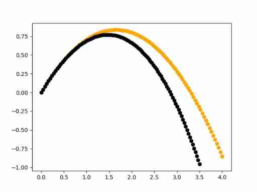

You can see , After adding air resistance , The speed of table tennis gradually decreases , It is no longer a beautiful parabola . It should be noted that , Here our trajectory is from y-z Side view from the plane .

Back to the top # The effect of adding a rotating arc circle

In the last chapter, we mainly considered the influence of air resistance on the trajectory of table tennis , The rotation of table tennis itself is not taken into account . Here we consider a loop ball scenario ： Add the trajectory of the arc circle or high hanging arc circle ball , It is necessary to add the upward rotation to the track of table tennis , Topspin will bring a downward Magnus force to table tennis , Make the arc of table tennis trajectory smaller . The specific form of Magnus force is referred to as follows Nasa Provided Kutta-Joukowski theory ：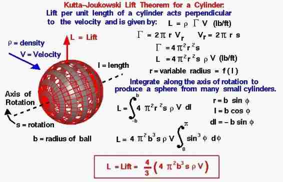

The relevant simulation code is as follows , For the convenience of calling , We wrap the module that generates the trajectory into a simple function ：

1
2
3
4
5
6
7
8
9
10
11
12
13
14
15
16
17
18
19
20
21
22
23
24
25
26
27
28
29
30
31
32
33
34
35
36
37
38
39
40
41
42
43
44
45
46
47
48
49
import numpy as np
from tqdm import trange
import matplotlib.pyplot as plt

vel = np.array([4.,4.])
vel0 = vel.copy()
steps = 100
r = 0.02
rho = 1.29
mass_min = 2.53e-03
mass_max = 2.70e-03
dt = 0.01
g = 9.8
C = 0.1
f0 = 0.
f1 = 0.
omega0 = 4
s0 = np.array([0.,0.])
s00 = np.array([0.,0.])

def F(vel, omega, r, rho):
    return 4*(4*np.pi**2*r**3*omega*vel*rho)/3

def Trace(steps, s0, vel0, f0, f1, dt, mass, omega0, r, rho, damping=False, KJ=False):
    s = [s0.copy()]
    tmps = s0.copy()
    for step in trange(steps):
        tmps += vel0*dt+0.5*f0*dt**2/mass
        s.append(tmps.copy())
        vel_norm = np.linalg.norm(vel0)
        if KJ:
            vel0 += np.array([np.sqrt(vel0[1]**2*(f0*dt/mass)**2/(vel0[0]**2+vel0[1]**2)),
                             -np.sqrt(vel0[0]**2*(f0*dt/mass)**2/(vel0[0]**2+vel0[1]**2))])
        if damping:
            vel0 -= np.array([f1*vel0[0]/vel_norm, f1*vel0[1]/vel_norm])*dt/mass
        vel0 += np.array([0.,-g])*dt
        f0 = F(np.linalg.norm(vel0), np.abs(omega0), r, rho)
        f1 = C*rho*np.pi*r**2*vel_norm**2
    return np.array(s)

s1 = Trace(steps, s0, vel0.copy(), f0, f1, dt, mass_min, omega0, r, rho, damping=False, KJ=False)
s2 = Trace(steps, s0, vel0.copy(), f0, f1, dt, mass_min, omega0, r, rho, damping=True, KJ=False)
s3 = Trace(steps, s0, vel0.copy(), f0, f1, dt, mass_min, omega0, r, rho, damping=True, KJ=True)

plt.figure()
plt.plot(s1[:,0], s1[:,1], 'o', color='orange')
plt.plot(s2[:,0], s2[:,1], 'o', color='black')
plt.plot(s3[:,0], s3[:,1], 'o', color='red')
plt.savefig('damping.png')

The operation results are as follows , The Yellow track indicates that the effect of air resistance and Magnus force is not considered , The black track indicates the result of considering air resistance without considering Magnus force , Relevant contents have been introduced in the previous chapter , Finally, there is a red track that shows the result of considering both air resistance and Magnus force , That is, the effect of the high hanging arc ball pulled out normally ：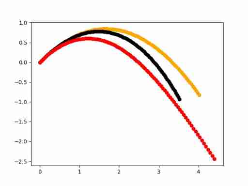

From this result we can learn that , The high hanging loop ball not only rotates strongly , It will also be more flat on the track , It is very threatening on the field .

Back to the top # Chopping curve

In the last chapter, we simulated the result of high hanging arc ball , That is to say, the upper rotating ball , And there is another non - arc playing method on the court ： Combination of cutting and attacking . The chopping technique , It can bring a strong downward rotation to the ball , That is to change the direction of mag's efforts , The relevant simulation code is as follows ：

1
2
3
4
5
6
7
8
9
10
11
12
13
14
15
16
17
18
19
20
21
22
23
24
25
26
27
28
29
30
31
32
33
34
35
36
37
38
39
40
41
42
43
44
45
46
47
48
49
50
51
52
import numpy as np
from tqdm import trange
import matplotlib.pyplot as plt

vel = np.array([4.,4.])
vel0 = vel.copy()
steps = 100
r = 0.02
rho = 1.29
mass_min = 2.53e-03
mass_max = 2.70e-03
dt = 0.01
g = 9.8
C = 0.1
f0 = 0.
f1 = 0.
omega0 = 4
s0 = np.array([0.,0.])
s00 = np.array([0.,0.])

def F(vel, omega, r, rho):
    return 4*(4*np.pi**2*r**3*omega*vel*rho)/3

def Trace(steps, s0, vel0, f0, f1, dt, mass, omega0, r, rho, damping=False, KJ=False, down\_spin=False):
    s = [s0.copy()]
    tmps = s0.copy()
    for step in trange(steps):
        tmps += vel0*dt+0.5*f0*dt**2/mass
        s.append(tmps.copy())
        vel_norm = np.linalg.norm(vel0)
        if KJ and not down_spin:
            vel0 += np.array([np.sqrt(vel0[1]**2*(f0*dt/mass)**2/(vel0[0]**2+vel0[1]**2)),
                              -np.sqrt(vel0[0]**2*(f0*dt/mass)**2/(vel0[0]**2+vel0[1]**2))])
        if KJ and down_spin:
            vel0 += np.array([-np.sqrt(vel0[1]**2*(f0*dt/mass)**2/(vel0[0]**2+vel0[1]**2)),
                              np.sqrt(vel0[0]**2*(f0*dt/mass)**2/(vel0[0]**2+vel0[1]**2))])
        if damping:
            vel0 -= np.array([f1*vel0[0]/vel_norm, f1*vel0[1]/vel_norm])*dt/mass
        vel0 += np.array([0.,-g])*dt
        f0 = F(np.linalg.norm(vel0), omega0, r, rho)
        f1 = C*rho*np.pi*r**2*vel_norm**2
    return np.array(s)

s1 = Trace(steps, s0, vel0.copy(), f0, f1, dt, mass_min, omega0, r, rho, damping=True, KJ=False)
s2 = Trace(steps, s0, vel0.copy(), f0, f1, dt, mass_min, omega0, r, rho, damping=True, KJ=True)
s3 = Trace(steps, s0, vel0.copy(), f0, f1, dt, mass_min, omega0, r, rho, damping=True, KJ=True, down_spin=True)

plt.figure()
plt.plot(s1[:,0], s1[:,1], 'o', color='orange')
plt.plot(s2[:,0], s2[:,1], 'o', color='black')
plt.plot(s3[:,0], s3[:,1], 'o', color='red')
plt.savefig('damping.png')

In this simulation , We compared it with no arc （ Orange track ）、 loop drive （ Black track ） And the chopping curve （ Red track ）, As shown in the figure below ：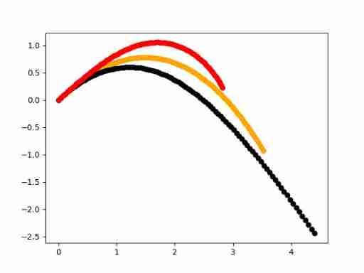

From the results, we find that , Due to the strong downward rotation, the table tennis brings the rising Magnus force , Therefore, the arc track of table tennis is lengthened , It is relatively easier to control the arc . For example, zhushihe , And Matt from the Chinese team , And the former national team's houyingli , They are all famous choppers .

Back to the top # Summary

In the previous blog, we introduced the simulation of table tennis arc technique with side spin , In this paper, we focus on the two track principles of high hanging arc and chopping arc , The influence of air resistance on the trajectory of table tennis is introduced . Through the simulation of air resistance and Magnus force , We can see different curves . For table tennis lovers , The results of this simulation , To develop strategies that may be used in the competition , For example, the low long arc ball 、 High short loop ball and so on . First, make a strategy from a scientific point of view , Then through daily training and consolidation, improve the technical level , Finally, it can be used in the official arena .

Back to the top # Copyright notice

The first link to this article is ：https://blog.csdn.net/dechinphy/p/damping.html

author ID：DechinPhy

For more original articles, please refer to ：https://blog.csdn.net/dechinphy/

Special link for reward ：https://blog.csdn.net/dechinphy/gallery/image/379634.html

Tencent cloud column synchronization ：https://cloud.tencent.com/developer/column/91958