Summary of some indicators for evaluating and selecting the best learning model

When evaluating models , Although accuracy is an important indicator of model evaluation and application model adjustment in the training stage , But it is not the best indicator for model evaluation , We can use several evaluation indicators to evaluate our model .

Because the data we use to build most models is unbalanced , And the model may be over fitted when training the data . In this paper , I will discuss and explain some of these methods , And give the use Python Examples of code .

Confusion matrix

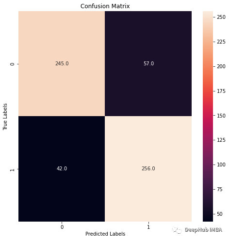
Using confusion matrix for classification model is a very good way to evaluate our model . It is very useful for visualizing the prediction results , Because the number of positive and negative test samples will be displayed . And it provides information about how the model interprets the predictions . Confusion matrix can be used for binary and multinomial classification . It consists of four matrices ：

#Import Libraries:
from random import random
from random import randint
import numpy as np
import pandas as pd
import matplotlib.pyplot as plt
import seaborn as sns
from sklearn.model_selection import train_test_split
from sklearn.linear_model import LogisticRegression
from sklearn.metrics import classification_report, confusion_matrix
from sklearn.metrics import precision_recall_curve
from sklearn.metrics import roc_curve

#Fabricating variables:
#Creating values for FeNO with 3 classes:
FeNO_0 = np.random.normal(15,20, 1000)
FeNO_1 = np.random.normal(35,20, 1000)
FeNO_2 = np.random.normal(65, 20, 1000)

#Creating values for FEV1 with 3 classes:
FEV1_0 = np.random.normal(4.50, 1, 1000)
FEV1_1 = np.random.uniform(3.75, 1.2, 1000)
FEV1_2 = np.random.uniform(2.35, 1.2, 1000)

#Creating values for Bronco Dilation with 3 classes:
BD_0 = np.random.normal(150,49, 1000)
BD_1 = np.random.uniform(250,50,1000)
BD_2 = np.random.uniform(350, 50, 1000)

#Creating labels variable with two classes (1)Disease (0)No disease:
no_disease = np.zeros((1500,), dtype=int)
disease = np.ones((1500,), dtype=int)

#Concatenate classes into one variable:
FeNO = np.concatenate([FeNO_0, FeNO_1, FeNO_2])
FEV1 = np.concatenate([FEV1_0, FEV1_1, FEV1_2])
BD = np.concatenate([BD_0, BD_1, BD_2])
dx = np.concatenate([not_asma, asma])

#Create DataFrame:
df = pd.DataFrame()#Add variables to DataFrame:
df['FeNO'] = FeNO.tolist()
df['FEV1'] = FEV1.tolist()
df['BD'] = BD.tolist()
df['dx'] = dx.tolist()

#Create X and y:
X = df.drop('dx', axis=1)
y = df['dx']#Train and Test split:
X_train, X_test, y_train, y_test = train_test_split(X, y, test_size=0.20)

#Build the model:
logisticregression = LogisticRegression().fit(X_train, y_train)

#Print accuracy metrics:
print("training set score: %f" % logisticregression.score(X_train, y_train))
print("test set score: %f" % logisticregression.score(X_test, y_test))

Now we can build the confusion matrix and examine our model :

# Predicting labels from X_test data
y_pred = logisticregression.predict(X_test)

# Create the confusion matrix
confmx = confusion_matrix(y_test, y_pred)
f, ax = plt.subplots(figsize = (8,8))
sns.heatmap(confmx, annot=True, fmt='.1f', ax = ax)
plt.xlabel('Predicted Labels')
plt.ylabel('True Labels')
plt.title('Confusion Matrix')
plt.show();

You can see , Model failed to 42 A label [1] and 57 A label [0] To classify .

The above method is the case of two categories , The steps of establishing a multi - class confusion matrix are similar .

#Fabricating variables:
#Creating values for FeNO with 3 classes:
FeNO_0 = np.random.normal(15,20, 1000)
FeNO_1 = np.random.normal(35,20, 1000)
FeNO_2 = np.random.normal(65, 20, 1000)

#Creating values for FEV1 with 3 classes:
FEV1_0 = np.random.normal(4.50, 1, 1000)
FEV1_1 = np.random.normal(3.75, 1.2, 1000)
FEV1_2 = np.random.normal(2.35, 1.2, 1000)

#Creating values for Broncho Dilation with 3 classes:
BD_0 = np.random.normal(150,49, 1000)
BD_1 = np.random.normal(250,50,1000)
BD_2 = np.random.normal(350, 50, 1000)

#Creating labels variable with three classes: 
no_disease = np.zeros((1000,), dtype=int)
possible_disease = np.ones((1000,), dtype=int)
disease = np.full((1000,), 2, dtype=int)

#Concatenate classes into one variable:
FeNO = np.concatenate([FeNO_0, FeNO_1, FeNO_2])
FEV1 = np.concatenate([FEV1_0, FEV1_1, FEV1_2])
BD = np.concatenate([BD_0, BD_1, BD_2])
dx = np.concatenate([no_disease, possible_disease, disease])

#Create DataFrame:
df = pd.DataFrame()

#Add variables to DataFrame:
df['FeNO'] = FeNO.tolist()
df['FEV1'] = FEV1.tolist()
df['BD'] = BD.tolist()
df['dx'] = dx.tolist()

#Creating X and y:
X = df.drop('dx', axis=1)
y = df['dx']#Data split into train and test:
X_train, X_test, y_train, y_test = train_test_split(X, y, test_size=0.20)#Fit Logistic Regression model:
logisticregression = LogisticRegression().fit(X_train, y_train)

#Evaluate Logistic Regression model:
print("training set score: %f" % logisticregression.score(X_train, y_train))
print("test set score: %f" % logisticregression.score(X_test, y_test))

Now let's create the confusion matrix

# Predicting labels from X_test data
y_pred = logisticregression.predict(X_test)

# Create the confusion matrix
confmx = confusion_matrix(y_test, y_pred)
f, ax = plt.subplots(figsize = (8,8))
sns.heatmap(confmx, annot=True, fmt='.1f', ax = ax)
plt.xlabel('Predicted Labels')
plt.ylabel('True Labels')
plt.title('Confusion Matrix')
plt.show();

By observing the confusion matrix , We can see the label [1] Has a higher error rate , So it is the most difficult to classify .

The evaluation index

In machine learning , There are many different metrics used to evaluate the performance of classifiers . The most common is :

• accuracy Accuracy: How good our model is in predicting results . This indicator is used to measure the closeness between the model output and the target results （ All samples predict the correct proportion ）.
• precision Precision: How many positive samples we predict are correct ? Precision rate （ It is predicted to be a positive sample , How many are actually positive samples , How many predicted positive samples are right ）
• Recall Recall: How many of our samples are target tags ? Recall rate （ How many positive samples have been predicted , How many of the positive samples can be predicted to be right ）
• **F1 Score:** Is the weighted average of precision and recall .

We still use the data and model built in the previous example to build the confusion matrix . Use sklearn It is very simple to print the evaluation indicators of the required model , So we use the existing functions directly here classification_report：

# Printing the model scores:
print(classification_report(y_test, y_pred))

You can see , label [0] More accurate , label [1] Of f1 Higher scores . In the confusion matrix of two classes , We see the label [1] Less misclassification data .

For multi label classification

# Printing the model scores:
print(classification_report(y_test, y_pred))

Through the confusion matrix , You can see the label [1] It's the hardest to classify , label [1] The accuracy of 、 Recall rate and f1 The score is the same .

ROC and AUC

ROC curve , Is a graphical representation , It shows the performance of the binary classifier system when its discrimination threshold changes .ROC The area under the curve is usually used to measure the usefulness of the test , A larger area means more useful testing .ROC The curve shows the false positive rate (FPR) And true positive rate (TPR) Comparison of .

#Get the values of FPR and TPR:
fpr, tpr, thresholds = roc_curve(y_test,logisticregression.decision_function(X_test))
plt.xlabel("FPR")
plt.ylabel("TPR (recall)")
plt.title("roc_curve");

# find threshold closest to zero:
close_zero = np.argmin(np.abs(thresholds))
plt.plot(fpr[close_zero], tpr[close_zero], 'o', markersize=10,
label="threshold zero", fillstyle="none", c='k', mew=2)
plt.legend(loc=4)

PR(precision recall ) curve

stay P-R In the curve ,Precision Abscissa ,Recall Vertical coordinates . stay ROC The more convex the curve in the curve, the better the upper left corner , stay P-R In the curve , The more convex the curve, the better the upper right corner .P-R The quality of the curve judgment model should be analyzed according to the specific situation , Some projects require a high recall rate 、 Some projects require high accuracy .P-R The drawing of the curve follows ROC The drawing of the curve is the same , At different thresholds, we get different Precision、Recall, Get a series of points , Put them in P-R It's drawn in the picture , And connect them in turn to get P-R chart .

PR A curve is just a graph ,y There's... On the shaft Precision value ,x There's... On the shaft Recall value . let me put it another way ,PR The curve is in y The shaft contains TP/(TP+FN), stay x The shaft contains TP/(TP+FP).

ROC The curve contains x On axis Recall = TPR = TP/(TP+FN) and y On axis FPR = FP/(FP+TN) Graph .ROC The curve does not realize the false positive rate and false negative rate , Instead, plot the true positive rate and the false positive rate .

PR Curves are often more common in problems involving information retrieval , Different scenes are right ROC and PRC Different preferences , We should treat them differently according to the actual situation .

#Get precision and recall thresholds:
precision, recall, thresholds = precision_recall_curve(y_test,logisticregression.decision_function(X_test))

# find threshold closest to zero:
close_zero = np.argmin(np.abs(thresholds))

#Plot curve:
plt.plot(precision[close_zero],     
         recall[close_zero], 
         'o', 
         markersize=10,
         label="threshold zero", 
         fillstyle="none", 
         c='k', 
         mew=2)
plt.plot(precision, recall, label="precision recall curve")
plt.xlabel("precision")
plt.ylabel("recall")
plt.title("precision_recall_curve");
plt.legend(loc="best")

https://avoid.overfit.cn/post/decf6f5fade44ffa98554368173062b0

author ：Carla Martins