Explain factor analysis in simple terms, with case teaching (full)

1、 effect

Factor analysis is based on the idea of dimension reduction , In the case of no or less loss of original data information as far as possible , The complex variables are aggregated into a few independent common factors , These common factors can reflect the main information of many variables , While reducing the number of variables , It also reflects the internal relationship between variables . Generally, factor analysis has three functions ： One is to reduce the dimension of factors , Second, calculate the factor weight , Third, calculate the weighted calculation factor to summarize the comprehensive score .

2、 Input / output description

Input ：2 Two or more quantitative variables （ Assuming that N A variable ）.
Output ： The minimum dimension reduction is 1 dimension （ A variable , Generally used for comprehensive evaluation ）, Maximum dimension reduction N A variable （ Generally used for data desensitization ）, At the same time, the composition weight of each variable after dimension reduction can be obtained , Used to represent the data retention of the original variable .

3、 Case example

According to the region 2021 Annual gross domestic product 、 Per capita disposable income and other indicators , Quantitatively evaluate the ranking of economic development level of multiple provinces, cities and regions or the weight of each index .

4、 Case data

Factor analysis data

5、 Case operation

Step1： New projects ;
Step2： Upload data ;
Step3： Select the corresponding data to open and preview , Click start analysis after confirmation ;

step4： choice 【 Factor analysis 】;
step5： View the corresponding data format ,【 Factor analysis 】 The input data is required to be put into [ ration ] The independent variables X（ Number of variables ≥2）.
step6： Select the number of principal components 、 Factor rotation mode （ Be careful ： In factor analysis, it tends to describe the correlation between the original variables , Therefore, in general, the number of principal components selected in factor analysis is the independent variable X Number , The feature root selection is based on the set threshold , The number of principal components larger than the corresponding limit is taken as the number of selected principal components , The default is 1.）
step7： Click on 【 To analyze 】, Complete the operation .

6、 Output results

Output results 1：KMO Inspection and Bartlett The test of

*p<0.05,**p<0.01,***p<0.001
Chart description ：KMO The results of the inspection show that ,KMO The value of is 0.775, meanwhile ,Bartlett Result display of spherical inspection , Significance P The value is 0.000***, The level is significant , Rejection of null hypothesis , That is to say, there is correlation between the variables , The results of factor analysis are valid , The reliability of the results was average .

Output results 2： Variance interpretation table

Chart description ：
The above table is the explanation table of total variance , It mainly depends on the contribution rate of factors to variable interpretation （ It can be understood as how many factors are needed to express the variable as 100%）, Generally speaking, it should be expressed to 90% That's all , Otherwise, adjust the number of factors . Variance explanation table , The contribution rate of cumulative interpretation of the first two factors reached 94.296%( Generally, it is greater than 90% that will do ）, It shows that the first two factors can be used to evaluate the economic development level of provinces, cities and regions . The first three factors are more effective , The contribution rate of cumulative interpretation reaches 98.921%.

Output results 3： Gravel map

Chart description ： When the broken line suddenly becomes smooth from steep , The number of principal components corresponding to steep to stable is the number of reference extracted principal components . It can be seen from the picture that , Start with the third principal component , The eigenvalues of the principal components begin to decrease slowly , The contribution to the cumulative interpretation of the factors reached 90% Under the circumstances , We can choose to keep the three principal components .

Output results 4： Factor load factor table

Chart description ：  The above table is the factor load factor table , The importance of hidden variables in each factor can be analyzed . The first factor and GDP 、 total imports and exports 、 Budgetary revenues 、 The four variables of current assets of industrial enterprises are highly correlated , Can be summed up as “ Local development status ”; The second factor is highly correlated with the variable of per capita disposable income , Can be summed up as “ People's affluence ”.

Output results 5： Factor load matrix thermodynamic diagram

Chart description ： The above figure shows the thermodynamic diagram of load matrix , The importance of hidden variables in each factor can be analyzed , The darker the color of the heat map, the greater the correlation . The first factor and GDP 、 total imports and exports 、 Budgetary revenues 、 The four variables of current assets of industrial enterprises are highly correlated , The second factor is highly correlated with the variable of per capita disposable income .

Output results 6： Factor load quadrant analysis

Chart description ： The factor load graph reduces the dimension of multiple factors into two or three factors , The spatial distribution of factors is presented by quadrant diagram . Make a two-dimensional factor load quadrant when two factors are retained . Three dimensional factor load quadrants are made when three factors are retained .

Output results 7： Composition matrix

Chart description ：  The formula of the model ：
F1=0.236× GDP ( One hundred million yuan )+0.057× Per capita disposable income ( element ）+0.192× total imports and exports ( Thousand dollars )+0.214× Budgetary revenues ( One hundred million yuan )+0.23× Current assets of industrial enterprises ( One hundred million yuan )
F2=0.244× GDP ( One hundred million yuan )+1.348× Per capita disposable income ( element ）+0.618× total imports and exports ( Thousand dollars )+0.552× Budgetary revenues ( One hundred million yuan )+0.298× Current assets of industrial enterprises ( One hundred million yuan )
F3=0.063× GDP ( One hundred million yuan )+0.821× Per capita disposable income ( element ）+4.519× total imports and exports ( Thousand dollars )+2.024× Budgetary revenues ( One hundred million yuan )+1.681× Current assets of industrial enterprises ( One hundred million yuan )
F4=-3.888× GDP ( One hundred million yuan )+0.164× Per capita disposable income ( element ）+0.517× total imports and exports ( Thousand dollars )-0.199× Budgetary revenues ( One hundred million yuan )+5.176× Current assets of industrial enterprises ( One hundred million yuan )
F5=-1.375× GDP ( One hundred million yuan )+0.605× Per capita disposable income ( element ）+0.94× total imports and exports ( Thousand dollars )+8.783× Budgetary revenues ( One hundred million yuan )-1.017× Current assets of industrial enterprises ( One hundred million yuan )
From above, we can get ： F=(0.669/1.0)×F1+(0.274/1.0)×F2+(0.046/1.0)×F3+(0.006/1.0)×F4+(0.005/1.0)×F5

Output results 8： Factor weight analysis

Chart description ：  The weight calculation result of the factor shows , factor 1 The weight for 66.9%、 factor 2 The weight for 27.396%、 factor 3 The weight for 4.625%、 factor 4 The weight for 0.576%、 factor 5 The weight for 0.503%.

Output results 9： Comprehensive score table

Chart description ： According to the comprehensive score , Guangdong Province has the highest comprehensive score , That is to say, the economic development level of Guangdong Province ranks first , The second is Jiangsu Province .

7、 matters needing attention

• Factor analysis requires strong collinearity or correlation between variables , Otherwise, it can't pass KMO Inspection and Bartlett Spherical test ;
• Factor analysis is a generalization of principal component analysis , Relative to principal component analysis , Prefer to describe the correlation between original variables （ Focus on analyzing the output results 4、 Output results 5、 Output results 6）.
• Factor analysis usually needs to integrate their own professional knowledge , And the software results , Even if the eigenvalue is less than 1, The principal components can also be extracted ;
• KMO The value is null There is no possible cause for ：

（1） Too little sample size will easily lead to too high correlation coefficient , It is generally expected that the analysis sample size is greater than 5 Times the number of analysis items ;
（2） The correlation between the analysis items is too high or too low .

8、 Model theory

Factor analysis is a method of reducing multidimensional variables to a few common factors according to the correlation between variables , Then the multidimensional variable statistical analysis method is analyzed . The basic idea is to divide the original variables into two parts : One part is the linear combination of common factors , Condensing represents most of the information in the original variables ; The other part is the special factor which has nothing to do with the common factor , It reflects the linear combination of common factors and original variables The gap between .p Dimension variable
x =[x1 ,…,xi ,…,xp ]T  The factor analysis model is :

  Or as

  among f =[f 1 ,f 2 ,…,f m ]T namely by carry take Of Male common because Son towards The amount , generation surface 了 primary beginning change The amount in No can straight Pick up view measuring but customer view save stay Of m (m <p) Three mutually independent common influencing factors ;A=（aik） Is the factor load matrix , matrix Elements aik by change The amount x i Yes Male common because Son fk The load of , It reflects the correlation coefficient between the two , The greater the absolute value , The more relevant ;
For multidimensional variables x The key to establish the factor analysis model is to solve the factor load matrix A  And the common factor vector  f , The steps are as follows ：
1） In order to eliminate the influence of different dimensions of variables , To contain n individual p Samples of dimensional variables X=[x1 ,x2 ,…,xn ] Standardize . After standardization , The mean value of each variable is 0, The variance of 1. For the convenience of expression, the standardized variables are still used  X  Express , Its elements are

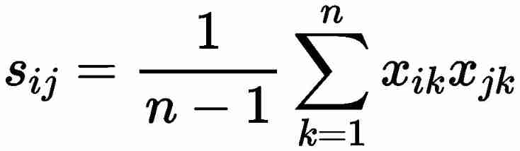
2） Find the covariance matrix of the sample  S , Its elements are

3） For the sample covariance matrix  S  Do eigenvalue decomposition , obtain p Eigenvalues λ1 ≥λ2≥…≥λp ≥0, The corresponding eigenvalue vector is γ1 , γ2 ,…,γp , Before taking it m The eigenvector of the largest eigenvalue estimates the factor load matrix . At the same time, in order to ensure the variance of each component of the common factor vector by 1, Divide it by the corresponding standard deviation λj . The corresponding eigenvector in the factor load matrix γj Then multiply by λj . Therefore, the factor load matrix

The parameter m Determined by the cumulative variance contribution rate of common factors , namely

It is generally believed , At present m The cumulative variance contribution rate of common factors exceeds 90% when , It can be considered that before m The linear combination of common factors can basically restore the original variable information .
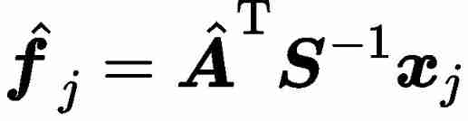
Common factor vector  f , That is, the specific score of the original variable on the common factor can be estimated by regression method

Go through the above steps , After obtaining the factor load matrix and the common factor vector , Then we can get that the special factor vector of the original variable is

9、 reference

[1] Gao Huixuan . Apply multivariate statistical analysis [M]. Beijing : Peking University press ,2005.
[2] Wenxu , Wang Hao , David , etc. . Identification method of abnormal data of bus load based on factor analysis [J]. Journal of Chongqing University ,2021,44(8):91-102.

10、 Learning Websites

SPSSPRO- Free professional online data analysis platform