当前位置:网站首页>CV learning notes - BP neural network training example (including detailed calculation process and formula derivation)
CV learning notes - BP neural network training example (including detailed calculation process and formula derivation)
2022-07-03 10:08:00 【Moresweet cat】
BP Examples of neural network training
1. BP neural network
About BP Neural network in my last blog 《CV Learning notes - Reasoning and training 》 Has been introduced in , I won't go into details here . Some of the things involved in this article are about BP The concept and basic knowledge of neural network are 《CV Learning notes - Reasoning and training 》 in , This article only deduces the process of examples .
BP The basic idea of Algorithm :
- Input the training set data into the input layer of neural network , Through the hidden layer , Finally, it reaches the output layer and outputs the results , This is the former
To the dissemination process . - Due to the error between the output result of neural network and the actual result , Then calculate the error between the estimated value and the actual value , And the error
Back propagation from the output layer to the hidden layer , Until it propagates to the input layer ; - In the process of back propagation , Adjust the values of various parameters according to the error ( The weight of connected neurons ), Make the total loss function minus
Small . - Iterate over the above three steps ( That is to train the data repeatedly ), Until the stop criteria are met .
2. Training examples
1. Example design
The green node is the first input layer , Each node represents a neuron , among i 1 i_1 i1、 i 2 i_2 i2 Represents the input value , b 1 b_1 b1 Is the offset value , The second layer contains h 1 h_1 h1 and h 2 h_2 h2 Two nodes , For the hidden layer , h 1 h_1 h1 and h 2 h_2 h2 Input value of neuron , b 2 b_2 b2 Is the offset value of the hidden layer , The third layer is the output layer , Include o 1 o_1 o1 and o 2 o_2 o2, w 1 w_1 w1~ w 8 w_8 w8 Is the weight between layers , Activate function using sigmoid function , The input value is [ i 1 = 0.05 , i 2 = 0.10 ] [i_1=0.05,i_2=0.10] [i1=0.05,i2=0.10], The correct output value is [ o 1 = 0.01 , o 2 = 0.99 ] [o_1=0.01,o_2=0.99] [o1=0.01,o2=0.99].
sigmoid Function is an activation function , In my last blog post 《CV Learning notes - Reasoning and training 》 Has been introduced in , No more details here .
![[ Failed to transfer the external chain picture , The origin station may have anti-theft chain mechanism , It is suggested to save the pictures and upload them directly (img-IZfBuEQM-1639470630420)(./imgs/image-20211214120357087.png)]](/img/9c/8424025d07e19a45c93ee15847d8be.jpg)
2. Training process
1. Forward propagation
Input layer -> Hidden layer :
According to the network structure diagram , Neuron h 1 h_1 h1 Receive the previous layer i 1 i_1 i1 and i 2 i_2 i2 As input , Use this input z h 1 z_{h1} zh1 Express , Then there are
z h 1 = w 1 × i 1 + w 2 × i 2 + b 1 × 1 = 0.15 × 0.05 + 0.2 × 0.1 + 0.35 × 1 = 0.3775 \begin{aligned} z_{h1}&=w_1\times i_1+w_2\times i_2 +b_1\times 1\\&=0.15\times0.05+0.2\times0.1+0.35\times 1\\&=0.3775 \end{aligned} zh1=w1×i1+w2×i2+b1×1=0.15×0.05+0.2×0.1+0.35×1=0.3775
Because the activation function is sigmoid function , So neurons h 1 h_1 h1 Output a h 1 a_{h1} ah1 by
a h 1 = 1 1 + e − z h 1 = 1 1 + e − 0.3775 = 0.593269992 a_{h1}=\frac{1}{1+e^{-z_{h1}}}=\frac{1}{1+e^{-0.3775}}=0.593269992 ah1=1+e−zh11=1+e−0.37751=0.593269992
The same can be , Neuron h 2 h_2 h2 Output a h 2 a_{h2} ah2 by
a h 2 = 0.596884378 a_{h2}=0.596884378 ah2=0.596884378
Hidden layer -> Output layer :
According to the network structure diagram , Neuron o 1 o_1 o1 The input of z o 1 z_{o1} zo1 From the previous layer h 1 h_1 h1 and h 2 h_2 h2 Weighted sum result of , so
z o 1 = w 5 × a h 1 + w 6 × a h 2 + b 2 × 1 = 0.4 × 0.593269992 + 0.45 × 0.596884378 + 0.6 × 1 = 1.105905967 \begin{aligned} z_{o1}&=w_5\times a_{h1}+w_6\times a_{h2}+b_2\times1\\&=0.4\times 0.593269992+0.45\times 0.596884378+0.6\times 1\\&=1.105905967 \end{aligned} zo1=w5×ah1+w6×ah2+b2×1=0.4×0.593269992+0.45×0.596884378+0.6×1=1.105905967
Similarly, we can calculate z o 2 z_{o2} zo2
Because of the use of the Internet sigmoid The function is the activation function , that o 1 o_1 o1 Output a o 1 a_{o1} ao1 by
a o 1 = 1 1 + e − z o 1 = 1 1 + e − 1.105905967 = 0.751365069 \begin{aligned} a_{o1}&=\frac{1}{1+e^{-z_{o1}}}\\&=\frac{1}{1+e^{-1.105905967}}\\&=0.751365069 \end{aligned} ao1=1+e−zo11=1+e−1.1059059671=0.751365069
Similarly, we can calculate a o 2 = 0.772928465 a_{o2}=0.772928465 ao2=0.772928465
thus , The output value of a complete forward propagation process is [ 0.751365069 , 0.772928465 ] [0.751365069,0.772928465] [0.751365069,0.772928465], And actual value [ 0.01 , 0.99 ] [0.01,0.99] [0.01,0.99] The error is quite large , Back propagation of errors is required , Recalculate after updating the weight .
2. Back propagation
Calculate the loss function :
The transfer error needs to be treated by the loss function , To estimate the appropriate transfer value for back-propagation and reasonably update the weight .
E t o t a l = ∑ 1 2 ( t a r g e t − o u t p u t ) 2 E o 1 = 1 2 ( 0.01 − 0.751365069 ) 2 = 0.274811083 E o 2 = 1 2 ( 0.99 − 0.772928465 ) 2 = 0.023560026 E t o t a l = E o 1 + E o 2 = 0.298371109 E_{total}=\sum\frac{1}{2}(target-output)^2\\ E_{o1}=\frac{1}{2}(0.01-0.751365069)^2=0.274811083\\ E_{o2}=\frac{1}{2}(0.99-0.772928465)^2=0.023560026\\ E_{total}=E_{o1}+E_{o2}=0.298371109 Etotal=∑21(target−output)2Eo1=21(0.01−0.751365069)2=0.274811083Eo2=21(0.99−0.772928465)2=0.023560026Etotal=Eo1+Eo2=0.298371109
Hidden layer -> Output layer weight update :
![[ Failed to transfer the external chain picture , The origin station may have anti-theft chain mechanism , It is suggested to save the pictures and upload them directly (img-65e1egtQ-1639470630421)(./imgs/image-20211214140502737.png)]](/img/f4/bea119a3a9302d7ef3b31bce52bbca.jpg)
With the weight parameter w 5 w_5 w5 For example , Use the overall loss to w 5 w_5 w5 After partial derivation, we can get w 5 w_5 w5 Contribution to the overall loss , namely
∂ E t o t a l ∂ w 5 = ∂ E t o t a l ∂ a o 1 × ∂ a o 1 ∂ z o 1 × ∂ z o 1 ∂ w 5 \frac{\partial E_{total}}{\partial w_5}=\frac{\partial E_{total}}{\partial a_{o1}}\times\frac{\partial a_{o1}}{\partial z_{o1}}\times\frac{\partial z_{o1}}{\partial w_5} ∂w5∂Etotal=∂ao1∂Etotal×∂zo1∂ao1×∂w5∂zo1
∂ E t o t a l ∂ E a o 1 \frac{\partial E_{total}}{\partial E_{a_{o1}}} ∂Eao1∂Etotal: Since the total loss is caused by two outputs ( a o 1 a_{o1} ao1 and a o 2 a_o2 ao2) It works out , Therefore, the overall loss can be on a o 1 、 a o 2 a_{o1}、a_{o2} ao1、ao2 Finding partial derivatives .
∂ a o 1 ∂ z o 1 \frac{\partial a_{o1}}{\partial z_{o1}} ∂zo1∂ao1: Due to output a o 1 a_{o1} ao1 It's input z o 1 z_{o1} zo1 adopt sigmoid Function is activated , so a o 1 a_{o1} ao1 It can be done to z o 1 z_{o1} zo1 Finding partial derivatives .
∂ z o 1 ∂ w 5 \frac{\partial z_{o1}}{\partial w_5} ∂w5∂zo1: because z o 1 z_{o1} zo1 It is from the previous network h 1 h_1 h1 The output of is based on the weight w 5 w_5 w5 Weighted sum results in , so z o 1 z_{o1} zo1 It can be done to w 5 w_5 w5 Finding partial derivatives .
Clear the relationship between the above formulas , w 5 w_5 w5 Contributed to z o 1 z_{o1} zo1, z o 1 z_{o1} zo1 Contributed to a o 1 a_{o1} ao1, and a o 1 a_{o1} ao1 Contributed again E t o t a l E_{total} Etotal, All hierarchical relationships are unique branches , Therefore, it is directly disassembled into the solution of the above formula , This hierarchical relationship is the hidden layer described in the following chapters -> The weight update process of the hidden layer will be a little more complicated .
After the above derivation , It can be calculated as :
∂ E t o t a l ∂ a o 1 \frac{\partial E_{total}}{\partial a_{o1}} ∂ao1∂Etotal :
E t o t a l = 1 2 ( t a r g e t o 1 − a o 1 ) 2 + 1 2 ( t a r g e t o 2 − a o 2 ) 2 ∂ E t o t a l ∂ a o 1 = 2 × 1 2 ( t a r g e t o 1 − a o 1 ) × ( − 1 ) = − ( t a r g e t o 1 − a o 1 ) = 0.751365069 − 0.01 = 0.741365069 \begin{aligned} E_{total}&=\frac{1}{2}(target_{o1}-a_{o1})^2+\frac{1}{2}(target_{o2}-a_{o2})^2\\ \frac{\partial E_{total}}{\partial a_{o1}}&=2\times\frac{1}{2}(target_{o1}-a_{o1})\times(-1)\\&=-(target_{o1}-a_{o1})\\&=0.751365069-0.01\\&=0.741365069 \end{aligned} Etotal∂ao1∂Etotal=21(targeto1−ao1)2+21(targeto2−ao2)2=2×21(targeto1−ao1)×(−1)=−(targeto1−ao1)=0.751365069−0.01=0.741365069
∂ a o 1 ∂ z o 1 \frac{\partial a_{o1}}{\partial z_{o1}} ∂zo1∂ao1:
a o 1 = 1 1 + e − z o 1 ∂ a o 1 ∂ z o 1 = a o 1 × ( 1 − a o 1 ) = 0.751365069 × ( 1 − 0.751365069 ) = 0.186815602 \begin{aligned} a_{o1}&=\frac{1}{1+e^{-z_{o1}}}\\ \frac{\partial a_{o1}}{\partial z_{o1}}&=a_{o1}\times(1-a_{o1})\\&=0.751365069\times(1-0.751365069)\\&=0.186815602 \end{aligned} ao1∂zo1∂ao1=1+e−zo11=ao1×(1−ao1)=0.751365069×(1−0.751365069)=0.186815602
∂ z o 1 ∂ w 5 \frac{\partial z_{o1}}{\partial w_5} ∂w5∂zo1:
z o 1 = w 5 × a h 1 + w 6 × a h 2 + b 2 × 1 ∂ z o 1 ∂ w 5 = a h 1 = 0.593269992 \begin{aligned} z_{o1}&=w_5\times a_{h1}+w_6\times a_{h2}+b_2\times1\\ \frac{\partial z_{o1}}{\partial w_5}&=a_{h1}\\&=0.593269992 \end{aligned} zo1∂w5∂zo1=w5×ah1+w6×ah2+b2×1=ah1=0.593269992
From the above three results , Available :
∂ E t o t a l ∂ w 5 = 0.741365069 × 0.186815602 × 0.593269992 = 0.082167041 \frac{\partial E_{total}}{\partial w_5}=0.741365069\times0.186815602\times0.593269992=0.082167041 ∂w5∂Etotal=0.741365069×0.186815602×0.593269992=0.082167041
If we remove specific values from the above steps , Abstract it out
Then we get
∂ E t o t a l ∂ w 5 = − ( t a r g e t o 1 − a o 1 ) × a o 1 × ( 1 − a o 1 ) × a h 1 ∂ E ∂ w j k = − ( t k − o k ) ⋅ s i g m o i d ( ∑ j w j k ⋅ o j ) ( I − s i g m o i d ( ∑ j w j k ⋅ o j ) ) ⋅ o j \frac{\partial E_{total}}{\partial w_5}=-(target_{o1}-a_{o1})\times a_{o1}\times(1-a_{o1})\times a_{h1}\\ \frac{\partial E}{\partial w_{jk}}=-(t_k-o_k)\cdot sigmoid(\sum_jw_{jk}\cdot o_j)(I-sigmoid(\sum_jw_{jk}\cdot o_j))\cdot o_j ∂w5∂Etotal=−(targeto1−ao1)×ao1×(1−ao1)×ah1∂wjk∂E=−(tk−ok)⋅sigmoid(j∑wjk⋅oj)(I−sigmoid(j∑wjk⋅oj))⋅oj
The formula in the second line was mentioned in my last blog , Now the derivation is made .
For the convenience of expression , use δ o 1 \delta_{o1} δo1 To represent the error of the output layer :
δ o 1 = ∂ E t o t a l ∂ a o 1 × ∂ a o 1 ∂ z o 1 = ∂ E t o t a l ∂ z o 1 δ o 1 = − ( t a r g e t o 1 − a o 1 ) × a o 1 × ( 1 − a o 1 ) \delta_{o1}=\frac{\partial E_{total}}{\partial a_{o1}}\times\frac{\partial a_{o1}}{\partial z_{o1}}=\frac{\partial E_{total}}{\partial z_{o1}}\\ \delta_{o1}=-(target_{o1}-a_{o1})\times a_{o1}\times(1-a_{o1}) δo1=∂ao1∂Etotal×∂zo1∂ao1=∂zo1∂Etotalδo1=−(targeto1−ao1)×ao1×(1−ao1)
Therefore, the overall loss for w 5 w_5 w5 The partial derivative of can be simply expressed as
∂ E t o t a l ∂ w 5 = δ o 1 × a h 1 \frac{\partial E_{total}}{\partial w_5}=\delta_{o1}\times a_{h1} ∂w5∂Etotal=δo1×ah1
be w 5 w_5 w5 The weight of is updated to :
w 5 + = w 5 − η × ∂ E t o t a l ∂ w 5 = 0.4 − 0.5 × 0.082167041 = 0.35891648 \begin{aligned} w_5^+&=w_5-\eta\times\frac{\partial E_{total}}{\partial w_5}\\&=0.4-0.5\times0.082167041\\&=0.35891648 \end{aligned} w5+=w5−η×∂w5∂Etotal=0.4−0.5×0.082167041=0.35891648
η \eta η For learning rate , In my last blog post 《CV Learning notes - Reasoning and training 》 Introduced in , I won't repeat .
Empathy , renewable w 6 , w 7 , w 8 w_6,w_7,w_8 w6,w7,w8:
w 6 + = 0.408666186 w 7 + = 0.511301270 w 8 + = 0.561370121 w_6^+=0.408666186\\ w_7^+=0.511301270\\ w_8^+=0.561370121 w6+=0.408666186w7+=0.511301270w8+=0.561370121
Hidden layer -> Update the weight of hidden layer :
![[ Failed to transfer the external chain picture , The origin station may have anti-theft chain mechanism , It is suggested to save the pictures and upload them directly (img-TZLCxQ3x-1639470630422)(./imgs/image-20211214151121680.png)]](/img/85/948ac192d006c3b0698a1eba6ff8bb.jpg)
Their ideas are roughly the same , But the difference is h 1 h_1 h1 Output a h 1 a_{h1} ah1 Yes E o 1 、 E o 2 E_{o1}、E_{o2} Eo1、Eo2 All have contributed , Therefore, the loss is generally right a h 1 a_{h1} ah1 When seeking partial derivative , According to the criterion of total differentiation , Be divided into pairs E o 1 、 E o 2 E_{o1}、E_{o2} Eo1、Eo2 Yes a h 1 a_{h1} ah1 Partial derivative of , namely
∂ E t o t a l ∂ w 1 = ∂ E t o t a l ∂ a h 1 × ∂ a h 1 ∂ z h 1 × ∂ z h 1 ∂ w 1 Its in : ∂ E t o t a l ∂ a h 1 = ∂ E o 1 ∂ a h 1 × ∂ E o 2 ∂ a h 1 \frac{\partial E_{total}}{\partial w_1}=\frac{\partial E_{total}}{\partial a_{h1}}\times\frac{\partial a_{h1}}{\partial z_{h1}}\times\frac{\partial z_{h1}}{\partial w_1}\\ among :\frac{\partial E_{total}}{\partial a_{h1}}=\frac{\partial E_{o1}}{\partial a_{h1}}\times\frac{\partial E_{o2}}{\partial a_{h1}} ∂w1∂Etotal=∂ah1∂Etotal×∂zh1∂ah1×∂w1∂zh1 Its in :∂ah1∂Etotal=∂ah1∂Eo1×∂ah1∂Eo2
From the above derivation , Calculated :
∂ E t o t a l ∂ a h 1 \frac{\partial E_{total}}{\partial a_{h1}} ∂ah1∂Etotal:
∂ E t o t a l ∂ a h 1 = ∂ E o 1 ∂ a h 1 × ∂ E o 2 ∂ a h 1 \frac{\partial E_{total}}{\partial a_{h1}}=\frac{\partial E_{o1}}{\partial a_{h1}}\times\frac{\partial E_{o2}}{\partial a_{h1}} ∂ah1∂Etotal=∂ah1∂Eo1×∂ah1∂Eo2
∂ E o 1 ∂ a h 1 \frac{\partial E_{o1}}{\partial a_{h1}} ∂ah1∂Eo1:
∂ E o 1 ∂ a h 1 = ∂ E o 1 ∂ a o 1 × ∂ a o 1 ∂ z o 1 × ∂ z o 1 ∂ a h 1 = 0.741365069 × 0.186815602 × 0.4 = 0.055399425 \begin{aligned} \frac{\partial E_{o1}}{\partial a_{h1}}&=\frac{\partial E_{o1}}{\partial a_{o1}}\times\frac{\partial a_{o1}}{\partial z_{o1}}\times\frac{\partial z_{o1}}{\partial a_{h1}}\\&=0.741365069\times0.186815602\times0.4\\&=0.055399425 \end{aligned} ∂ah1∂Eo1=∂ao1∂Eo1×∂zo1∂ao1×∂ah1∂zo1=0.741365069×0.186815602×0.4=0.055399425
The same can be :
∂ E o 2 ∂ a h 1 = − 0.019049119 \frac{\partial E_{o2}}{\partial a_{h1}}=-0.019049119 ∂ah1∂Eo2=−0.019049119
The two add up to :
∂ E t o t a l ∂ a h 1 = ∂ E o 1 ∂ a h 1 × ∂ E o 2 ∂ a h 1 = 0.055399435 − 0.019049119 = 0.036350306 \begin{aligned} \frac{\partial E_{total}}{\partial a_{h1}}&=\frac{\partial E_{o1}}{\partial a_{h1}}\times\frac{\partial E_{o2}}{\partial a_{h1}}\\&=0.055399435-0.019049119\\&=0.036350306 \end{aligned} ∂ah1∂Etotal=∂ah1∂Eo1×∂ah1∂Eo2=0.055399435−0.019049119=0.036350306
∂ a h 1 ∂ z h 1 \frac{\partial a_{h1}}{\partial z_{h1}} ∂zh1∂ah1:
∂ a h 1 ∂ z h 1 = a h 1 × ( 1 − a h 1 ) = 0.593269992 × ( 1 − 0.593269992 ) = 0.2413007086 \begin{aligned} \frac{\partial a_{h1}}{\partial z_{h1}}&=a_{h1}\times(1-a_{h1})\\&=0.593269992\times(1-0.593269992)\\&=0.2413007086 \end{aligned} ∂zh1∂ah1=ah1×(1−ah1)=0.593269992×(1−0.593269992)=0.2413007086
∂ z h 1 ∂ w 1 \frac{\partial z_{h1}}{\partial w_1} ∂w1∂zh1:
∂ z h 1 ∂ w 1 = i 1 = 0.05 \frac{\partial z_{h1}}{\partial w_1}=i_1=0.05 ∂w1∂zh1=i1=0.05
final result :
∂ E t o t a l ∂ w 1 = 0.036350306 × 0.2413007086 × 0.05 = 0.000438568 \frac{\partial E_{total}}{\partial w_1}=0.036350306\times0.2413007086\times0.05=0.000438568 ∂w1∂Etotal=0.036350306×0.2413007086×0.05=0.000438568
The simplified method in the previous section , use δ h 1 \delta_{h1} δh1 Represents hidden layer cells h 1 h_1 h1 The error of the :
∂ E t o t a l ∂ w 1 = ( ∑ i ∂ E t o t a l ∂ a i × ∂ a i ∂ z i × ∂ z i ∂ a h 1 ) × ∂ a h 1 ∂ z h 1 × ∂ z h 1 ∂ w 1 = ( ∑ i δ i × w h i ) × a h 1 × ( 1 − a h 1 ) × i 1 = δ h 1 × i 1 \begin{aligned} \frac{\partial E_{total}}{\partial w_1}&=(\sum_i\frac{\partial E_{total}}{\partial a_{i}}\times\frac{\partial a_{i}}{\partial z_{i}}\times\frac{\partial z_{i}}{\partial a_{h1}})\times\frac{\partial a_{h1}}{\partial z_{h1}}\times\frac{\partial z_{h1}}{\partial w_1}\\&=(\sum_i\delta_i\times w_{hi})\times a_{h1}\times(1-a_{h1})\times i_1\\&=\delta_{h_1}\times i_1 \end{aligned} ∂w1∂Etotal=(i∑∂ai∂Etotal×∂zi∂ai×∂ah1∂zi)×∂zh1∂ah1×∂w1∂zh1=(i∑δi×whi)×ah1×(1−ah1)×i1=δh1×i1
w 1 w_1 w1 The weight of is updated to :
w 1 + = w 1 − η × ∂ E t o t a l ∂ w 1 = 0.15 − 0.5 × 0.000438568 = 0.149780716 w_1^+=w_1-\eta\times\frac{\partial E_{total}}{\partial w_1}=0.15-0.5\times0.000438568=0.149780716 w1+=w1−η×∂w1∂Etotal=0.15−0.5×0.000438568=0.149780716
Empathy , to update w 2 , w 3 , w 4 w_2,w_3,w_4 w2,w3,w4:
w 2 + = 0.19956143 w 3 + = 0.24975114 w 4 + = 0.29950229 w_2^+=0.19956143\\ w_3^+=0.24975114\\ w_4^+=0.29950229 w2+=0.19956143w3+=0.24975114w4+=0.29950229
thus , The process of a back propagation ends .
This is how the training process iterates , Error after forward propagation , Update weights in back propagation , Then forward propagation , This goes on over and over again , After the first iteration of this example, the total error is from 0.298371109 Down to 0.291027924, In iteration 10000 Next time , The total error is reduced to 0.000035085. Output is [0.015912196,0.984065734]
Personal study notes , Just learn to communicate , Reprint please indicate the source !
边栏推荐
- 2312. Selling wood blocks | things about the interviewer and crazy Zhang San (leetcode, with mind map + all solutions)
- The data read by pandas is saved to the MySQL database
- Gpiof6, 7, 8 configuration
- Liquid crystal display
- Swing transformer details-1
- 自動裝箱與拆箱了解嗎?原理是什麼?
- Dynamic layout management
- Open Euler Kernel Technology Sharing - Issue 1 - kdump Basic Principles, use and Case Introduction
- LeetCode - 703 数据流中的第 K 大元素(设计 - 优先队列)
- Emballage automatique et déballage compris? Quel est le principe?
猜你喜欢
2.Elment Ui 日期选择器 格式化问题
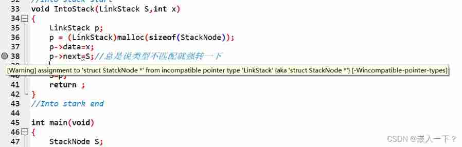
Assignment to '*' form incompatible pointer type 'linkstack' {aka '*'} problem solving
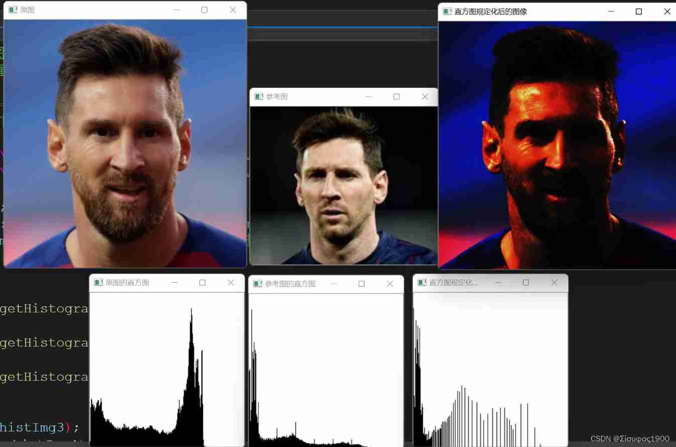
Opencv gray histogram, histogram specification

Seven sorting of ten thousand words by hand (code + dynamic diagram demonstration)

CV learning notes - feature extraction

03 FastJson 解决循环引用

MySQL root user needs sudo login

RESNET code details

Pycharm cannot import custom package
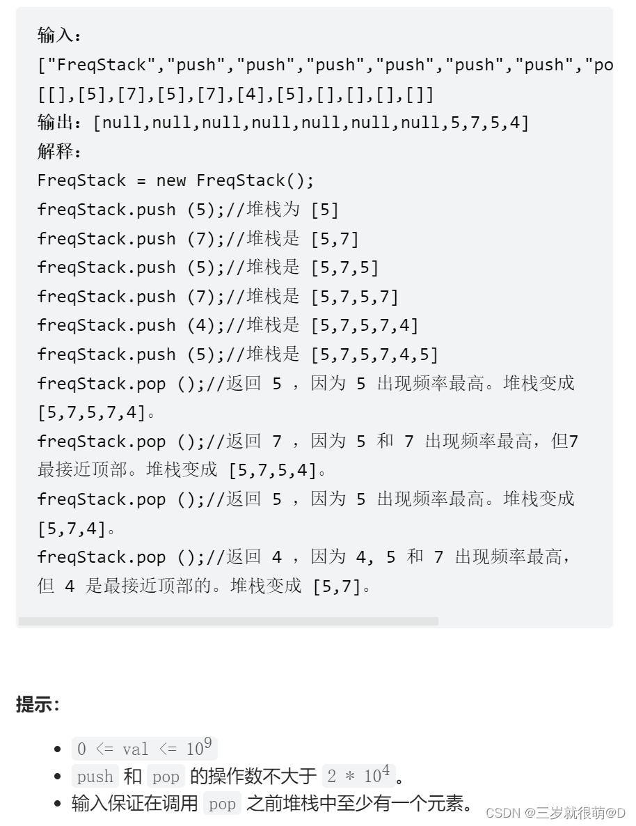
Leetcode - 895 maximum frequency stack (Design - hash table + priority queue hash table + stack)*
随机推荐
[combinatorics] combinatorial existence theorem (three combinatorial existence theorems | finite poset decomposition theorem | Ramsey theorem | existence theorem of different representative systems |
Vscode markdown export PDF error
Seven sorting of ten thousand words by hand (code + dynamic diagram demonstration)
Toolbutton property settings
Leetcode 300 longest ascending subsequence
getopt_ Typical use of long function
My 4G smart charging pile gateway design and development related articles
Yocto technology sharing phase IV: customize and add software package support
byte alignment
2. Elment UI date selector formatting problem
Opencv Harris corner detection
I think all friends should know that the basic law of learning is: from easy to difficult
Application of 51 single chip microcomputer timer
Leetcode bit operation
Design of charging pile mqtt transplantation based on 4G EC20 module
Do you understand automatic packing and unpacking? What is the principle?
Connect Alibaba cloud servers in the form of key pairs
SCM is now overwhelming, a wide variety, so that developers are overwhelmed
STM32 general timer output PWM control steering gear
CV learning notes - feature extraction