当前位置:网站首页>pytroch、tensorflow对比学习—搭建模型范式(低阶、中阶、高阶API示例)
pytroch、tensorflow对比学习—搭建模型范式(低阶、中阶、高阶API示例)
2022-08-01 04:57:00 【卖香油的少掌柜】
搭建模型范式(低阶、中阶、高阶API示例)
前言
本文是《pytorch-tensorflow-Comparative study》,pytorch和tensorflow对比学习专栏,第四章——搭建模型范式(低阶、中阶、高阶API示例)。
虽然说这两个框架在语法和接口的命名上有很多地方是不同的,但是深度学习的建模过程确实基本上都是一个套路的。
所以该笔记的笔记方式是:在使用相同的处理功能模块上,对比记录pytorch和tensorflow两者的API接口,和语法。
1,有利于深入理解深度学习建模过程流程。
2,有利于理解pytorch,和tensorflow设计上的不同,更加灵活的使用在自己的项目中。
3,有利于深入理解各个功能模块的使用。
本章节主要对比学习pytorch 和tensorflow有关搭建模型范式(低阶、中阶、高阶API示例)接口,和语法。

低阶API示例
这里范例使用Pytorch和tensorflow的低阶API分别实现线性回归模型和DNN二分类模型。
低阶API主要包括张量操作,计算图和自动微分。
先定义打印时间函数(在中介和高阶API示例中都会使用到):
pytorch
import os
import datetime

#打印时间
def printbar():
    nowtime = datetime.datetime.now().strftime('%Y-%m-%d %H:%M:%S')
    print("\n"+"=========="*8 + "%s"%nowtime)

#mac系统上pytorch和matplotlib在jupyter中同时跑需要更改环境变量
os.environ["KMP_DUPLICATE_LIB_OK"]="TRUE"
tensorflow
import tensorflow as tf

#打印时间分割线
@tf.function
def printbar():
    today_ts = tf.timestamp()%(24*60*60)

    hour = tf.cast(today_ts//3600+8,tf.int32)%tf.constant(24)
    minite = tf.cast((today_ts%3600)//60,tf.int32)
    second = tf.cast(tf.floor(today_ts%60),tf.int32)

    def timeformat(m):
        if tf.strings.length(tf.strings.format("{}",m))==1:
            return(tf.strings.format("0{}",m))
        else:
            return(tf.strings.format("{}",m))

    timestring = tf.strings.join([timeformat(hour),timeformat(minite),
                timeformat(second)],separator = ":")
    tf.print("=========="*8+timestring)
线性回归模型
准备数据
pytorch
import numpy as np
import pandas as pd
from matplotlib import pyplot as plt
import torch
from torch import nn
#样本数量
n = 400
# 生成测试用数据集
X = 10*torch.rand([n,2])-5.0 #torch.rand是均匀分布
w0 = torch.tensor([[2.0],[-3.0]])
b0 = torch.tensor([[10.0]])
Y = [email protected] + b0 + torch.normal( 0.0,2.0,size = [n,1]) # @表示矩阵乘法,增加正态扰动
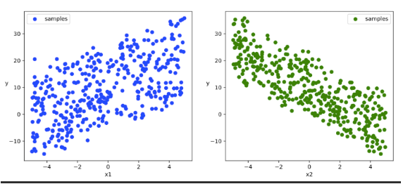
# 数据可视化
plt.figure(figsize = (12,5))
ax1 = plt.subplot(121)
ax1.scatter(X[:,0].numpy(),Y[:,0].numpy(), c = "b",label = "samples")
ax1.legend()
plt.xlabel("x1")
plt.ylabel("y",rotation = 0)
ax2 = plt.subplot(122)
ax2.scatter(X[:,1].numpy(),Y[:,0].numpy(), c = "g",label = "samples")
ax2.legend()
plt.xlabel("x2")
plt.ylabel("y",rotation = 0)
plt.show()
tensorflow
import numpy as np
import pandas as pd
from matplotlib import pyplot as plt
import tensorflow as tf
#样本数量
n = 400
# 生成测试用数据集
X = tf.random.uniform([n,2],minval=-10,maxval=10)
w0 = tf.constant([[2.0],[-3.0]])
b0 = tf.constant([[3.0]])
Y = [email protected] + b0 + tf.random.normal([n,1],mean = 0.0,stddev= 2.0) # @表示矩阵乘法,增加正态扰动
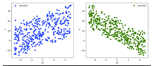
# 数据可视化
plt.figure(figsize = (12,5))
ax1 = plt.subplot(121)
ax1.scatter(X[:,0],Y[:,0], c = "b")
plt.xlabel("x1")
plt.ylabel("y",rotation = 0)
ax2 = plt.subplot(122)
ax2.scatter(X[:,1],Y[:,0], c = "g")
plt.xlabel("x2")
plt.ylabel("y",rotation = 0)
plt.show()
数据管道
pytroch
# 构建数据管道迭代器
def data_iter(features, labels, batch_size=8):
    num_examples = len(features)
    indices = list(range(num_examples))
    np.random.shuffle(indices)  #样本的读取顺序是随机的
    for i in range(0, num_examples, batch_size):
        indexs = torch.LongTensor(indices[i: min(i + batch_size, num_examples)])
        yield  features.index_select(0, indexs), labels.index_select(0, indexs)

# 测试数据管道效果
batch_size = 8
(features,labels) = next(data_iter(X,Y,batch_size))
print(features)
print(labels)
# tensor([[-4.3880, 1.3655],
# [-0.1082, 3.9533],
# [-2.6286, 2.7058],
# [ 1.0604, -1.8646],
# [-1.5805, 1.5406],
# [-2.6217, -3.2342],
# [ 2.3748, -0.6449],
# [-1.2478, -2.0509]])
# tensor([[-0.2069],
# [-3.2494],
# [-6.9620],
# [17.0528],
# [ 1.1076],
# [17.2117],
# [16.1081],
# [14.7092]])
tensorflow
# 构建数据管道迭代器
def data_iter(features, labels, batch_size=8):
    num_examples = len(features)
    indices = list(range(num_examples))
    np.random.shuffle(indices)  #样本的读取顺序是随机的
    for i in range(0, num_examples, batch_size):
        indexs = indices[i: min(i + batch_size, num_examples)]
        yield tf.gather(features,indexs), tf.gather(labels,indexs)

# 测试数据管道效果
batch_size = 8
(features,labels) = next(data_iter(X,Y,batch_size))
print(features)
print(labels)
# tf.Tensor(
# [[ 2.6161194 0.11071014]
# [ 9.79207 -0.70180416]
# [ 9.792343 6.9149055 ]
# [-2.4186516 -9.375019 ]
# [ 9.83749 -3.4637213 ]
# [ 7.3953056 4.374569 ]
# [-0.14686584 -0.28063297]
# [ 0.49001217 -9.739792 ]], shape=(8, 2), dtype=float32)
# tf.Tensor(
# [[ 9.334667 ]
# [22.058844 ]
# [ 3.0695205]
# [26.736238 ]
# [35.292133 ]
# [ 4.2943544]
# [ 1.6713585]
# [34.826904 ]], shape=(8, 1), dtype=float32)
定义模型
pytorch
# 定义模型
class LinearRegression:

    def __init__(self):
        self.w = torch.randn_like(w0,requires_grad=True)
        self.b = torch.zeros_like(b0,requires_grad=True)

    #正向传播
    def forward(self,x):
        return [email protected].w + self.b

    # 损失函数
    def loss_func(self,y_pred,y_true):
        return torch.mean((y_pred - y_true)**2/2)

model = LinearRegression()
tensorflow
w = tf.Variable(tf.random.normal(w0.shape))
b = tf.Variable(tf.zeros_like(b0,dtype = tf.float32))

# 定义模型
class LinearRegression:
    #正向传播
    def __call__(self,x):
        return [email protected] + b

    # 损失函数
    def loss_func(self,y_true,y_pred):
        return tf.reduce_mean((y_true - y_pred)**2/2)

model = LinearRegression()
训练模型
def train_step(model, features, labels):

    predictions = model.forward(features)
    loss = model.loss_func(predictions,labels)

    # 反向传播求梯度
    loss.backward()

    # 使用torch.no_grad()避免梯度记录,也可以通过操作 model.w.data 实现避免梯度记录
    with torch.no_grad():
        # 梯度下降法更新参数
        model.w -= 0.001*model.w.grad
        model.b -= 0.001*model.b.grad

        # 梯度清零
        model.w.grad.zero_()
        model.b.grad.zero_()
    return loss
# 测试train_step效果
batch_size = 10
(features,labels) = next(data_iter(X,Y,batch_size))
train_step(model,features,labels)
# tensor(92.8199, grad_fn=<MeanBackward0>)
def train_model(model,epochs):
    for epoch in range(1,epochs+1):
        for features, labels in data_iter(X,Y,10):
            loss = train_step(model,features,labels)

        if epoch%200==0:
            printbar()
            print("epoch =",epoch,"loss = ",loss.item())
            print("model.w =",model.w.data)
            print("model.b =",model.b.data)

train_model(model,epochs = 1000)

# ================================================================================2020-07-05 08:27:57
# epoch = 200 loss = 2.6340413093566895
# model.w = tensor([[ 2.0283],
# [-2.9632]])
# model.b = tensor([[10.0748]])
#
# ================================================================================2020-07-05 08:28:00
# epoch = 400 loss = 2.24908709526062
# model.w = tensor([[ 2.0300],
# [-2.9643]])
# model.b = tensor([[10.0781]])#
# ....
tensorflow
''' ##使用autograph机制转换成静态图加速 @tf.function '''
# 使用动态图调试
def train_step(model, features, labels):
    with tf.GradientTape() as tape:
        predictions = model(features)
        loss = model.loss_func(labels, predictions)
    # 反向传播求梯度
    dloss_dw,dloss_db = tape.gradient(loss,[w,b])
    # 梯度下降法更新参数
    w.assign(w - 0.001*dloss_dw)
    b.assign(b - 0.001*dloss_db)

    return loss
# 测试train_step效果
batch_size = 10
(features,labels) = next(data_iter(X,Y,batch_size))
train_step(model,features,labels)
# <tf.Tensor: shape=(), dtype=float32, numpy=211.09982>
def train_model(model,epochs):
    for epoch in tf.range(1,epochs+1):
        for features, labels in data_iter(X,Y,10):
            loss = train_step(model,features,labels)

        if epoch%50==0:
            printbar()
            tf.print("epoch =",epoch,"loss = ",loss)
            tf.print("w =",w)
            tf.print("b =",b)

train_model(model,epochs = 200)

# ================================================================================16:35:56
# epoch = 50 loss = 1.78806472
# w = [[1.97554708]
# [-2.97719598]]
# b = [[2.60692883]]
# ================================================================================16:36:00
# epoch = 100 loss = 2.64588404
# w = [[1.97319281]
# [-2.97810626]]
# b = [[2.95525956]]
# ...
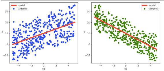
结果可视化
# 结果可视化

plt.figure(figsize = (12,5))
ax1 = plt.subplot(121)
ax1.scatter(X[:,0].numpy(),Y[:,0].numpy(), c = "b",label = "samples")
ax1.plot(X[:,0].numpy(),(model.w[0].data*X[:,0]+model.b[0].data).numpy(),"-r",linewidth = 5.0,label = "model")
ax1.legend()
plt.xlabel("x1")
plt.ylabel("y",rotation = 0)

ax2 = plt.subplot(122)
ax2.scatter(X[:,1].numpy(),Y[:,0].numpy(), c = "g",label = "samples")
ax2.plot(X[:,1].numpy(),(model.w[1].data*X[:,1]+model.b[0].data).numpy(),"-r",linewidth = 5.0,label = "model")
ax2.legend()
plt.xlabel("x2")
plt.ylabel("y",rotation = 0)

plt.show()
DNN二分类模型
准备数据
pytorch
import numpy as np
import pandas as pd
from matplotlib import pyplot as plt
import torch
from torch import nn
%matplotlib inline
%config InlineBackend.figure_format = 'svg'

#正负样本数量
n_positive,n_negative = 2000,2000

#生成正样本, 小圆环分布
r_p = 5.0 + torch.normal(0.0,1.0,size = [n_positive,1])
theta_p = 2*np.pi*torch.rand([n_positive,1])
Xp = torch.cat([r_p*torch.cos(theta_p),r_p*torch.sin(theta_p)],axis = 1)
Yp = torch.ones_like(r_p)

#生成负样本, 大圆环分布
r_n = 8.0 + torch.normal(0.0,1.0,size = [n_negative,1])
theta_n = 2*np.pi*torch.rand([n_negative,1])
Xn = torch.cat([r_n*torch.cos(theta_n),r_n*torch.sin(theta_n)],axis = 1)
Yn = torch.zeros_like(r_n)

#汇总样本
X = torch.cat([Xp,Xn],axis = 0)
Y = torch.cat([Yp,Yn],axis = 0)


#可视化
plt.figure(figsize = (6,6))
plt.scatter(Xp[:,0].numpy(),Xp[:,1].numpy(),c = "r")
plt.scatter(Xn[:,0].numpy(),Xn[:,1].numpy(),c = "g")
plt.legend(["positive","negative"]);

tensorflow
import numpy as np
import pandas as pd
from matplotlib import pyplot as plt
import tensorflow as tf
%matplotlib inline
%config InlineBackend.figure_format = 'svg'

#正负样本数量
n_positive,n_negative = 2000,2000

#生成正样本, 小圆环分布
r_p = 5.0 + tf.random.truncated_normal([n_positive,1],0.0,1.0)
theta_p = tf.random.uniform([n_positive,1],0.0,2*np.pi)
Xp = tf.concat([r_p*tf.cos(theta_p),r_p*tf.sin(theta_p)],axis = 1)
Yp = tf.ones_like(r_p)

#生成负样本, 大圆环分布
r_n = 8.0 + tf.random.truncated_normal([n_negative,1],0.0,1.0)
theta_n = tf.random.uniform([n_negative,1],0.0,2*np.pi)
Xn = tf.concat([r_n*tf.cos(theta_n),r_n*tf.sin(theta_n)],axis = 1)
Yn = tf.zeros_like(r_n)

#汇总样本
X = tf.concat([Xp,Xn],axis = 0)
Y = tf.concat([Yp,Yn],axis = 0)


#可视化
plt.figure(figsize = (6,6))
plt.scatter(Xp[:,0].numpy(),Xp[:,1].numpy(),c = "r")
plt.scatter(Xn[:,0].numpy(),Xn[:,1].numpy(),c = "g")
plt.legend(["positive","negative"]);

数据管道
pytorch
# 构建数据管道迭代器
def data_iter(features, labels, batch_size=8):
    num_examples = len(features)
    indices = list(range(num_examples))
    np.random.shuffle(indices)  #样本的读取顺序是随机的
    for i in range(0, num_examples, batch_size):
        indexs = torch.LongTensor(indices[i: min(i + batch_size, num_examples)])
        yield  features.index_select(0, indexs), labels.index_select(0, indexs)

# 测试数据管道效果
batch_size = 8
(features,labels) = next(data_iter(X,Y,batch_size))
print(features)
print(labels)
# tensor([[ 6.9914, -1.0820],
# [ 4.8156, 4.0532],
# [-1.0697, -7.4644],
# [ 2.6291, 3.8851],
# [-1.6780, -4.3390],
# [-6.1495, 1.2269],
# [-4.3422, 3.9552],
# [-6.2265, 2.6159]])
# tensor([[0.],
# [1.],
# [0.],
# [1.],
# [1.],
# [1.],
# [1.],
# [1.]])
tensorflow
# 构建数据管道迭代器
def data_iter(features, labels, batch_size=8):
    num_examples = len(features)
    indices = list(range(num_examples))
    np.random.shuffle(indices)  #样本的读取顺序是随机的
    for i in range(0, num_examples, batch_size):
        indexs = indices[i: min(i + batch_size, num_examples)]
        yield tf.gather(features,indexs), tf.gather(labels,indexs)

# 测试数据管道效果
batch_size = 10
(features,labels) = next(data_iter(X,Y,batch_size))
print(features)
print(labels)
# tf.Tensor(
# [[ 0.03732629 3.5783494 ]
# [ 0.542919 5.035079 ]
# [ 5.860281 -2.4476354 ]
# [ 0.63657564 3.194231 ]
# [-3.5072308 2.5578873 ]
# [-2.4109735 -3.6621518 ]
# [ 4.0975413 -2.4172943 ]
# [ 1.9393908 -6.782317 ]
# [-4.7453732 -0.5176727 ]
# [-1.4057113 -7.9775257 ]], shape=(10, 2), dtype=float32)
# tf.Tensor(
# [[1.]
# [1.]
# [0.]
# [1.]
# [1.]
# [1.]
# [1.]
# [0.]
# [1.]
# [0.]], shape=(10, 1), dtype=float32)
定义模型
pythorch
此处范例我们利用nn.Module来组织模型变量。
class DNNModel(nn.Module):
    def __init__(self):
        super(DNNModel, self).__init__()
        self.w1 = nn.Parameter(torch.randn(2,4))
        self.b1 = nn.Parameter(torch.zeros(1,4))
        self.w2 = nn.Parameter(torch.randn(4,8))
        self.b2 = nn.Parameter(torch.zeros(1,8))
        self.w3 = nn.Parameter(torch.randn(8,1))
        self.b3 = nn.Parameter(torch.zeros(1,1))

    # 正向传播
    def forward(self,x):
        x = torch.relu([email protected].w1 + self.b1)
        x = torch.relu([email protected].w2 + self.b2)
        y = torch.sigmoid([email protected].w3 + self.b3)
        return y

    # 损失函数(二元交叉熵)
    def loss_func(self,y_pred,y_true):
        #将预测值限制在1e-7以上, 1- (1e-7)以下,避免log(0)错误
        eps = 1e-7
        y_pred = torch.clamp(y_pred,eps,1.0-eps)
        bce = - y_true*torch.log(y_pred) - (1-y_true)*torch.log(1-y_pred)
        return torch.mean(bce)

    # 评估指标(准确率)
    def metric_func(self,y_pred,y_true):
        y_pred = torch.where(y_pred>0.5,torch.ones_like(y_pred,dtype = torch.float32),
                          torch.zeros_like(y_pred,dtype = torch.float32))
        acc = torch.mean(1-torch.abs(y_true-y_pred))
        return acc

model = DNNModel()
# 测试模型结构
batch_size = 10
(features,labels) = next(data_iter(X,Y,batch_size))

predictions = model(features)

loss = model.loss_func(labels,predictions)
metric = model.metric_func(labels,predictions)

print("init loss:", loss.item())
print("init metric:", metric.item())
# init loss: 7.979694366455078
# init metric: 0.50347900390625

len(list(model.parameters()))
# 6
tensorflow
此处范例我们利用tf.Module来组织模型变量,关于tf.Module的较详细介绍参考本书第四章最后一节: Autograph和tf.Module。
class DNNModel(tf.Module):
    def __init__(self,name = None):
        super(DNNModel, self).__init__(name=name)
        self.w1 = tf.Variable(tf.random.truncated_normal([2,4]),dtype = tf.float32)
        self.b1 = tf.Variable(tf.zeros([1,4]),dtype = tf.float32)
        self.w2 = tf.Variable(tf.random.truncated_normal([4,8]),dtype = tf.float32)
        self.b2 = tf.Variable(tf.zeros([1,8]),dtype = tf.float32)
        self.w3 = tf.Variable(tf.random.truncated_normal([8,1]),dtype = tf.float32)
        self.b3 = tf.Variable(tf.zeros([1,1]),dtype = tf.float32)


    # 正向传播
    @tf.function(input_signature=[tf.TensorSpec(shape = [None,2], dtype = tf.float32)])
    def __call__(self,x):
        x = tf.nn.relu([email protected].w1 + self.b1)
        x = tf.nn.relu([email protected].w2 + self.b2)
        y = tf.nn.sigmoid([email protected].w3 + self.b3)
        return y

    # 损失函数(二元交叉熵)
    @tf.function(input_signature=[tf.TensorSpec(shape = [None,1], dtype = tf.float32),
                              tf.TensorSpec(shape = [None,1], dtype = tf.float32)])
    def loss_func(self,y_true,y_pred):
        #将预测值限制在 1e-7 以上, 1 - 1e-7 以下,避免log(0)错误
        eps = 1e-7
        y_pred = tf.clip_by_value(y_pred,eps,1.0-eps)
        bce = - y_true*tf.math.log(y_pred) - (1-y_true)*tf.math.log(1-y_pred)
        return  tf.reduce_mean(bce)

    # 评估指标(准确率)
    @tf.function(input_signature=[tf.TensorSpec(shape = [None,1], dtype = tf.float32),
                              tf.TensorSpec(shape = [None,1], dtype = tf.float32)])
    def metric_func(self,y_true,y_pred):
        y_pred = tf.where(y_pred>0.5,tf.ones_like(y_pred,dtype = tf.float32),
                          tf.zeros_like(y_pred,dtype = tf.float32))
        acc = tf.reduce_mean(1-tf.abs(y_true-y_pred))
        return acc

model = DNNModel()
# 测试模型结构
batch_size = 10
(features,labels) = next(data_iter(X,Y,batch_size))

predictions = model(features)

loss = model.loss_func(labels,predictions)
metric = model.metric_func(labels,predictions)

tf.print("init loss:",loss)
tf.print("init metric",metric)
# init loss: 1.76568353
# init metric 0.6
print(len(model.trainable_variables))
# 6
训练模型
pytorch
def train_step(model, features, labels):

    # 正向传播求损失
    predictions = model.forward(features)
    loss = model.loss_func(predictions,labels)
    metric = model.metric_func(predictions,labels)

    # 反向传播求梯度
    loss.backward()

    # 梯度下降法更新参数
    for param in model.parameters():
        #注意是对param.data进行重新赋值,避免此处操作引起梯度记录
        param.data = (param.data - 0.01*param.grad.data)

    # 梯度清零
    model.zero_grad()

    return loss.item(),metric.item()


def train_model(model,epochs):
    for epoch in range(1,epochs+1):
        loss_list,metric_list = [],[]
        for features, labels in data_iter(X,Y,20):
            lossi,metrici = train_step(model,features,labels)
            loss_list.append(lossi)
            metric_list.append(metrici)
        loss = np.mean(loss_list)
        metric = np.mean(metric_list)

        if epoch%100==0:
            printbar()
            print("epoch =",epoch,"loss = ",loss,"metric = ",metric)

train_model(model,epochs = 1000)
# ================================================================================2020-07-05 08:32:16
# epoch = 100 loss = 0.24841043589636683 metric = 0.8944999960064888
#
# ================================================================================2020-07-05 08:32:34
# epoch = 200 loss = 0.20398724960163236 metric = 0.920999992787838
#
# ================================================================================2020-07-05 08:32:54
# epoch = 300 loss = 0.19509393003769218 metric = 0.9239999914169311
#
# ================================================================================2020-07-05 08:33:14
# ...
tensorflow
##使用autograph机制转换成静态图加速

@tf.function
def train_step(model, features, labels):

    # 正向传播求损失
    with tf.GradientTape() as tape:
        predictions = model(features)
        loss = model.loss_func(labels, predictions)

    # 反向传播求梯度
    grads = tape.gradient(loss, model.trainable_variables)

    # 执行梯度下降
    for p, dloss_dp in zip(model.trainable_variables,grads):
        p.assign(p - 0.001*dloss_dp)

    # 计算评估指标
    metric = model.metric_func(labels,predictions)

    return loss, metric


def train_model(model,epochs):
    for epoch in tf.range(1,epochs+1):
        for features, labels in data_iter(X,Y,100):
            loss,metric = train_step(model,features,labels)
        if epoch%100==0:
            printbar()
            tf.print("epoch =",epoch,"loss = ",loss, "accuracy = ", metric)


train_model(model,epochs = 600)

# ================================================================================16:47:35
# epoch = 100 loss = 0.567795336 accuracy = 0.71
# ================================================================================16:47:39
# epoch = 200 loss = 0.50955683 accuracy = 0.77
# ================================================================================16:47:43
# epoch = 300 loss = 0.421476126 accuracy = 0.84
结果可视化
fig, (ax1,ax2) = plt.subplots(nrows=1,ncols=2,figsize = (12,5))
ax1.scatter(Xp[:,0],Xp[:,1], c="r")
ax1.scatter(Xn[:,0],Xn[:,1],c = "g")
ax1.legend(["positive","negative"]);
ax1.set_title("y_true");

Xp_pred = X[torch.squeeze(model.forward(X)>=0.5)]
Xn_pred = X[torch.squeeze(model.forward(X)<0.5)]

ax2.scatter(Xp_pred[:,0],Xp_pred[:,1],c = "r")
ax2.scatter(Xn_pred[:,0],Xn_pred[:,1],c = "g")
ax2.legend(["positive","negative"]);
ax2.set_title("y_pred");

中介API示例
Pytorch的中阶API主要包括各种模型层,损失函数,优化器,数据管道等等。
TensorFlow的中阶API主要包括各种模型层,损失函数,优化器,数据管道,特征列等等。
线性回归模型
准备数据
pytroch和tensorflow 的数据准备和低阶API部分相同,使用相同的数据,可以直接把代码粘过来,这里不做重复。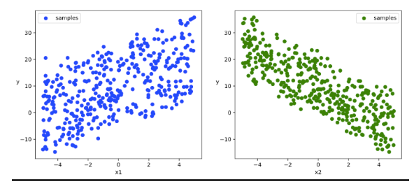
数据管道
pytroch
#构建输入数据管道
ds = TensorDataset(X,Y)
dl = DataLoader(ds,batch_size = 10,shuffle=True,num_workers=2)
tensorflow
#构建输入数据管道
ds = tf.data.Dataset.from_tensor_slices((X,Y)) \
     .shuffle(buffer_size = 100).batch(10) \
     .prefetch(tf.data.experimental.AUTOTUNE)
定义模型
pytroch
model = nn.Linear(2,1) #线性层

model.loss_func = nn.MSELoss()
model.optimizer = torch.optim.SGD(model.parameters(),lr = 0.01)
tensorflow
model = layers.Dense(units = 1)
model.build(input_shape = (2,)) #用build方法创建variables
model.loss_func = losses.mean_squared_error
model.optimizer = optimizers.SGD(learning_rate=0.001)
训练模型
pytorch
def train_step(model, features, labels):

    predictions = model(features)
    loss = model.loss_func(predictions,labels)
    loss.backward()
    model.optimizer.step()
    model.optimizer.zero_grad()
    return loss.item()

# 测试train_step效果
features,labels = next(iter(dl))
train_step(model,features,labels)
# 269.98016357421875
def train_model(model,epochs):
    for epoch in range(1,epochs+1):
        for features, labels in dl:
            loss = train_step(model,features,labels)
        if epoch%50==0:
            printbar()
            w = model.state_dict()["weight"]
            b = model.state_dict()["bias"]
            print("epoch =",epoch,"loss = ",loss)
            print("w =",w)
            print("b =",b)
train_model(model,epochs = 200)

# ================================================================================2020-07-05 22:51:53
# epoch = 50 loss = 3.0177409648895264
# w = tensor([[ 1.9315, -2.9573]])
# b = tensor([9.9625])
#
# ================================================================================2020-07-05 22:51:57
# epoch = 100 loss = 2.1144354343414307
# w = tensor([[ 1.9760, -2.9398]])
# b = tensor([9.9428])
# ...
tensorflow
#使用autograph机制转换成静态图加速

@tf.function
def train_step(model, features, labels):
    with tf.GradientTape() as tape:
        predictions = model(features)
        loss = model.loss_func(tf.reshape(labels,[-1]), tf.reshape(predictions,[-1]))
    grads = tape.gradient(loss,model.variables)
    model.optimizer.apply_gradients(zip(grads,model.variables))
    return loss

# 测试train_step效果
features,labels = next(ds.as_numpy_iterator())
train_step(model,features,labels)
def train_model(model,epochs):
    for epoch in tf.range(1,epochs+1):
        loss = tf.constant(0.0)
        for features, labels in ds:
            loss = train_step(model,features,labels)
        if epoch%50==0:
            printbar()
            tf.print("epoch =",epoch,"loss = ",loss)
            tf.print("w =",model.variables[0])
            tf.print("b =",model.variables[1])
train_model(model,epochs = 200)
# ===========================================================================17:01:48
# epoch = 50 loss = 2.56481647
# w = [[1.99355531]
# [-2.99061537]]
# b = [3.09484935]
# ===========================================================================17:01:51
# epoch = 100 loss = 5.96198225
# w = [[1.98028314]
# [-2.96975136]]
# b = [3.09501529]
# ...
结果可视化
代码同上章节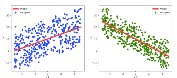
DNN二分类模型
准备数据
pytroch和tensorflow 的数据准备和低阶API部分相同,使用相同的数据,可以直接把代码粘过来,这里不做重复。
数据管道
pytorch
#构建输入数据管道
ds = TensorDataset(X,Y)
dl = DataLoader(ds,batch_size = 10,shuffle=True,num_workers=2)
tensorflow
#构建输入数据管道
ds = tf.data.Dataset.from_tensor_slices((X,Y)) \
     .shuffle(buffer_size = 4000).batch(100) \
     .prefetch(tf.data.experimental.AUTOTUNE)
定义模型
pytroch
class DNNModel(nn.Module):
    def __init__(self):
        super(DNNModel, self).__init__()
        self.fc1 = nn.Linear(2,4)
        self.fc2 = nn.Linear(4,8)
        self.fc3 = nn.Linear(8,1)

    # 正向传播
    def forward(self,x):
        x = F.relu(self.fc1(x))
        x = F.relu(self.fc2(x))
        y = nn.Sigmoid()(self.fc3(x))
        return y

    # 损失函数
    def loss_func(self,y_pred,y_true):
        return nn.BCELoss()(y_pred,y_true)

    # 评估函数(准确率)
    def metric_func(self,y_pred,y_true):
        y_pred = torch.where(y_pred>0.5,torch.ones_like(y_pred,dtype = torch.float32),
                          torch.zeros_like(y_pred,dtype = torch.float32))
        acc = torch.mean(1-torch.abs(y_true-y_pred))
        return acc

    # 优化器
    @property
    def optimizer(self):
        return torch.optim.Adam(self.parameters(),lr = 0.001)

model = DNNModel()
# 测试模型结构
(features,labels) = next(iter(dl))
predictions = model(features)

loss = model.loss_func(predictions,labels)
metric = model.metric_func(predictions,labels)

print("init loss:",loss.item())
print("init metric:",metric.item())
# init loss: 0.7065666913986206
# init metric: 0.6000000238418579
tensorflow
class DNNModel(tf.Module):
    def __init__(self,name = None):
        super(DNNModel, self).__init__(name=name)
        self.dense1 = layers.Dense(4,activation = "relu")
        self.dense2 = layers.Dense(8,activation = "relu")
        self.dense3 = layers.Dense(1,activation = "sigmoid")


    # 正向传播
    @tf.function(input_signature=[tf.TensorSpec(shape = [None,2], dtype = tf.float32)])
    def __call__(self,x):
        x = self.dense1(x)
        x = self.dense2(x)
        y = self.dense3(x)
        return y

model = DNNModel()
model.loss_func = losses.binary_crossentropy
model.metric_func = metrics.binary_accuracy
model.optimizer = optimizers.Adam(learning_rate=0.001)
# 测试模型结构
(features,labels) = next(ds.as_numpy_iterator())

predictions = model(features)

loss = model.loss_func(tf.reshape(labels,[-1]),tf.reshape(predictions,[-1]))
metric = model.metric_func(tf.reshape(labels,[-1]),tf.reshape(predictions,[-1]))

tf.print("init loss:",loss)
tf.print("init metric",metric)
# init loss: 1.13653195
# init metric 0.5
训练模型
pytroch
def train_step(model, features, labels):

    # 正向传播求损失
    predictions = model(features)
    loss = model.loss_func(predictions,labels)
    metric = model.metric_func(predictions,labels)

    # 反向传播求梯度
    loss.backward()

    # 更新模型参数
    model.optimizer.step()
    model.optimizer.zero_grad()

    return loss.item(),metric.item()

# 测试train_step效果
features,labels = next(iter(dl))
train_step(model,features,labels)
# (0.6048880815505981, 0.699999988079071)
def train_model(model,epochs):
    for epoch in range(1,epochs+1):
        loss_list,metric_list = [],[]
        for features, labels in dl:
            lossi,metrici = train_step(model,features,labels)
            loss_list.append(lossi)
            metric_list.append(metrici)
        loss = np.mean(loss_list)
        metric = np.mean(metric_list)

        if epoch%100==0:
            printbar()
            print("epoch =",epoch,"loss = ",loss,"metric = ",metric)

train_model(model,epochs = 300)
# ==============================================================2020-07-05 22:56:38
# epoch = 100 loss = 0.23532892110607917 metric = 0.934749992787838
#
# ==============================================================2020-07-05 22:58:18
# epoch = 200 loss = 0.24743918558603128 metric = 0.934999993443489
tensorflow
#使用autograph机制转换成静态图加速

@tf.function
def train_step(model, features, labels):
    with tf.GradientTape() as tape:
        predictions = model(features)
        loss = model.loss_func(tf.reshape(labels,[-1]), tf.reshape(predictions,[-1]))
    grads = tape.gradient(loss,model.trainable_variables)
    model.optimizer.apply_gradients(zip(grads,model.trainable_variables))

    metric = model.metric_func(tf.reshape(labels,[-1]), tf.reshape(predictions,[-1]))

    return loss,metric

# 测试train_step效果
features,labels = next(ds.as_numpy_iterator())
train_step(model,features,labels)
# (<tf.Tensor: shape=(), dtype=float32, numpy=1.2033114>,
# <tf.Tensor: shape=(), dtype=float32, numpy=0.47>)
def train_model(model,epochs):
    for epoch in tf.range(1,epochs+1):
        loss, metric = tf.constant(0.0),tf.constant(0.0)
        for features, labels in ds:
            loss,metric = train_step(model,features,labels)
        if epoch%10==0:
            printbar()
            tf.print("epoch =",epoch,"loss = ",loss, "accuracy = ",metric)
train_model(model,epochs = 60)

# ========================================================================17:07:36
# epoch = 10 loss = 0.556449413 accuracy = 0.79
# ========================================================================17:07:38
# epoch = 20 loss = 0.439187407 accuracy = 0.86
# ...
结果可视化
代码同上章节
高阶API示例
TensorFlow的高阶API主要为tf.keras.models提供的模型的类接口。
使用Keras接口有以下3种方式构建模型:使用Sequential按层顺序构建模型,使用函数式API构建任意结构模型,继承Model基类构建自定义模型。
此处分别演示使用Sequential按层顺序构建模型以及继承Model基类构建自定义模型。
Pytorch没有官方的高阶API,一般需要用户自己实现训练循环、验证循环、和预测循环。
不过有大神通过仿照tf.keras.Model的功能对Pytorch的nn.Module进行了封装,设计了torchkeras.Model类,
实现了 fit, validate,predict, summary 方法,相当于用户自定义高阶API。
并示范了用它实现线性回归模型。
此外,还通过借用pytorch_lightning的功能,封装了类Keras接口的另外一种实现,即torchkeras.LightModel类。
pytorch
此范例我们通过继承torchkeras.Model模型接口,实现线性回归模型。
tensorflow
此范例我们使用Sequential按层顺序构建模型,并使用内置model.fit方法训练模型【面向新手】。
线性回归模型
准备数据
代码同上章节
数据管道
pytroch
#构建输入数据管道
ds = TensorDataset(X,Y)
ds_train,ds_valid = torch.utils.data.random_split(ds,[int(400*0.7),400-int(400*0.7)])
dl_train = DataLoader(ds_train,batch_size = 10,shuffle=True,num_workers=2)
dl_valid = DataLoader(ds_valid,batch_size = 10,num_workers=2)
tensorflow
数据管道的构建继承在高阶API训练阶段的参数上
定义模型
pytorch
# 继承用户自定义模型
from torchkeras import Model
class LinearRegression(Model):
    def __init__(self):
        super(LinearRegression, self).__init__()
        self.fc = nn.Linear(2,1)

    def forward(self,x):
        return self.fc(x)

model = LinearRegression()
model.summary(input_shape = (2,))
""" ---------------------------------------------------------------- Layer (type) Output Shape Param # ================================================================ Linear-1 [-1, 1] 3 ================================================================ Total params: 3 Trainable params: 3 Non-trainable params: 0 ---------------------------------------------------------------- Input size (MB): 0.000008 Forward/backward pass size (MB): 0.000008 Params size (MB): 0.000011 Estimated Total Size (MB): 0.000027 ---------------------------------------------------------------- """
tensorflow
tf.keras.backend.clear_session()

model = models.Sequential()
model.add(layers.Dense(1,input_shape =(2,)))
model.summary()
"""" Model: "sequential" _________________________________________________________________ Layer (type) Output Shape Param # ================================================================= dense (Dense) (None, 1) 3 ================================================================= Total params: 3 Trainable params: 3 Non-trainable params: 0 """
训练模型
pytroch
### 使用fit方法进行训练

def mean_absolute_error(y_pred,y_true):
    return torch.mean(torch.abs(y_pred-y_true))

def mean_absolute_percent_error(y_pred,y_true):
    absolute_percent_error = (torch.abs(y_pred-y_true)+1e-7)/(torch.abs(y_true)+1e-7)
    return torch.mean(absolute_percent_error)

model.compile(loss_func = nn.MSELoss(),
              optimizer= torch.optim.Adam(model.parameters(),lr = 0.01),
              metrics_dict={
    "mae":mean_absolute_error,"mape":mean_absolute_percent_error})

dfhistory = model.fit(200,dl_train = dl_train, dl_val = dl_valid,log_step_freq = 20)
"""
Start Training ...

================================================================================2020-07-05 23:07:25
{'step': 20, 'loss': 226.768, 'mae': 12.198, 'mape': 1.212}

 +-------+---------+-------+-------+----------+---------+----------+
| epoch |   loss  |  mae  |  mape | val_loss | val_mae | val_mape |
+-------+---------+-------+-------+----------+---------+----------+
|   1   | 230.773 | 12.41 | 1.394 | 223.262  |  12.582 |  1.095   |
+-------+---------+-------+-------+----------+---------+----------+

================================================================================2020-07-05 23:07:26
{'step': 20, 'loss': 200.964, 'mae': 11.584, 'mape': 1.382}

 +-------+---------+--------+------+----------+---------+----------+
| epoch |   loss  |  mae   | mape | val_loss | val_mae | val_mape |
+-------+---------+--------+------+----------+---------+----------+
|   2   | 206.238 | 11.759 | 1.26 | 199.669  |  11.895 |  1.012   |
+-------+---------+--------+------+----------+---------+----------+
...
“”“
tensorflow
### 使用fit方法进行训练

model.compile(optimizer="adam",loss="mse",metrics=["mae"])
model.fit(X,Y,batch_size = 10,epochs = 200)

tf.print("w = ",model.layers[0].kernel)
tf.print("b = ",model.layers[0].bias)
Epoch 197/200
400/400 [==============================] - 0s 190us/sample - loss: 4.3977 - mae: 1.7129
Epoch 198/200
400/400 [==============================] - 0s 172us/sample - loss: 4.3918 - mae: 1.7117
Epoch 199/200
400/400 [==============================] - 0s 134us/sample - loss: 4.3861 - mae: 1.7106
Epoch 200/200
400/400 [==============================] - 0s 166us/sample - loss: 4.3786 - mae: 1.7092
w =  [[1.99339032]
 [-3.00866461]]
b =  [2.67018795]
结果可视化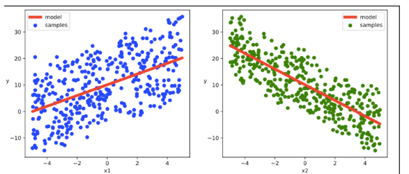
DNN二分类模型
pytorch中:此范例我们通过继承torchkeras.LightModel模型接口,实现DNN二分类模型。
**tensorflow中:**此范例我们使用继承Model基类构建自定义模型,并构建自定义训练循环【面向专家】
准备数据
代码同上章节

数据管道
pytorch
ds = TensorDataset(X,Y)

ds_train,ds_valid = torch.utils.data.random_split(ds,[int(len(ds)*0.7),len(ds)-int(len(ds)*0.7)])
dl_train = DataLoader(ds_train,batch_size = 100,shuffle=True,num_workers=2)
dl_valid = DataLoader(ds_valid,batch_size = 100,num_workers=2)
tensorflow
ds_train = tf.data.Dataset.from_tensor_slices((X[0:n*3//4,:],Y[0:n*3//4,:])) \
     .shuffle(buffer_size = 1000).batch(20) \
     .prefetch(tf.data.experimental.AUTOTUNE) \
     .cache()

ds_valid = tf.data.Dataset.from_tensor_slices((X[n*3//4:,:],Y[n*3//4:,:])) \
     .batch(20) \
     .prefetch(tf.data.experimental.AUTOTUNE) \
     .cache()
定义模型
pytorch
class Net(nn.Module):
    def __init__(self):
        super().__init__()
        self.fc1 = nn.Linear(2,4)
        self.fc2 = nn.Linear(4,8)
        self.fc3 = nn.Linear(8,1)

    def forward(self,x):
        x = F.relu(self.fc1(x))
        x = F.relu(self.fc2(x))
        y = nn.Sigmoid()(self.fc3(x))
        return y

class Model(torchkeras.LightModel):

    #loss,and optional metrics
    def shared_step(self,batch)->dict:
        x, y = batch
        prediction = self(x)
        loss = nn.BCELoss()(prediction,y)
        preds = torch.where(prediction>0.5,torch.ones_like(prediction),torch.zeros_like(prediction))
        acc = pl.metrics.functional.accuracy(preds, y)
        # attention: there must be a key of "loss" in the returned dict
        dic = {
    "loss":loss,"acc":acc}
        return dic

    #optimizer,and optional lr_scheduler
    def configure_optimizers(self):
        optimizer = torch.optim.Adam(self.parameters(), lr=1e-2)
        lr_scheduler = torch.optim.lr_scheduler.StepLR(optimizer, step_size=10, gamma=0.0001)
        return {
    "optimizer":optimizer,"lr_scheduler":lr_scheduler}

pl.seed_everything(1234)
net = Net()
model = Model(net)


torchkeras.summary(model,input_shape =(2,))
----------------------------------------------------------------
        Layer (type)               Output Shape         Param #
================================================================
            Linear-1                    [-1, 4]              12
            Linear-2                    [-1, 8]              40
            Linear-3                    [-1, 1]               9
================================================================
Total params: 61
Trainable params: 61
Non-trainable params: 0
----------------------------------------------------------------
Input size (MB): 0.000008
Forward/backward pass size (MB): 0.000099
Params size (MB): 0.000233
Estimated Total Size (MB): 0.000340
----------------------------------------------------------------
tensorflow
tf.keras.backend.clear_session()
class DNNModel(models.Model):
    def __init__(self):
        super(DNNModel, self).__init__()

    def build(self,input_shape):
        self.dense1 = layers.Dense(4,activation = "relu",name = "dense1")
        self.dense2 = layers.Dense(8,activation = "relu",name = "dense2")
        self.dense3 = layers.Dense(1,activation = "sigmoid",name = "dense3")
        super(DNNModel,self).build(input_shape)

    # 正向传播
    @tf.function(input_signature=[tf.TensorSpec(shape = [None,2], dtype = tf.float32)])
    def call(self,x):
        x = self.dense1(x)
        x = self.dense2(x)
        y = self.dense3(x)
        return y

model = DNNModel()
model.build(input_shape =(None,2))

model.summary()
Model: "dnn_model"
_________________________________________________________________
Layer (type)                 Output Shape              Param #
=================================================================
dense1 (Dense)               multiple                  12
_________________________________________________________________
dense2 (Dense)               multiple                  40
_________________________________________________________________
dense3 (Dense)               multiple                  9
=================================================================
Total params: 61
Trainable params: 61
Non-trainable params: 0
_________________________________________________________________
训练模型
pytroch
ckpt_cb = pl.callbacks.ModelCheckpoint(monitor='val_loss')

# set gpus=0 will use cpu,
# set gpus=1 will use 1 gpu
# set gpus=2 will use 2gpus
# set gpus = -1 will use all gpus
# you can also set gpus = [0,1] to use the given gpus
# you can even set tpu_cores=2 to use two tpus

trainer = pl.Trainer(max_epochs=100,gpus = 0, callbacks=[ckpt_cb])

trainer.fit(model,dl_train,dl_valid)
=============================================================2021-01-16 23:41:38
epoch =  0
{'val_loss': 0.6706896424293518, 'val_acc': 0.5558333396911621}
{'acc': 0.5157142281532288, 'loss': 0.6820458769798279}

============================================================2021-01-16 23:41:39
epoch =  1
{'val_loss': 0.653035581111908, 'val_acc': 0.5708333849906921}
{'acc': 0.5457143783569336, 'loss': 0.6677185297012329}
...
tensorflow
### 自定义训练循环

optimizer = optimizers.Adam(learning_rate=0.01)
loss_func = tf.keras.losses.BinaryCrossentropy()

train_loss = tf.keras.metrics.Mean(name='train_loss')
train_metric = tf.keras.metrics.BinaryAccuracy(name='train_accuracy')

valid_loss = tf.keras.metrics.Mean(name='valid_loss')
valid_metric = tf.keras.metrics.BinaryAccuracy(name='valid_accuracy')


@tf.function
def train_step(model, features, labels):
    with tf.GradientTape() as tape:
        predictions = model(features)
        loss = loss_func(labels, predictions)
    grads = tape.gradient(loss, model.trainable_variables)
    optimizer.apply_gradients(zip(grads, model.trainable_variables))

    train_loss.update_state(loss)
    train_metric.update_state(labels, predictions)

@tf.function
def valid_step(model, features, labels):
    predictions = model(features)
    batch_loss = loss_func(labels, predictions)
    valid_loss.update_state(batch_loss)
    valid_metric.update_state(labels, predictions)


def train_model(model,ds_train,ds_valid,epochs):
    for epoch in tf.range(1,epochs+1):
        for features, labels in ds_train:
            train_step(model,features,labels)

        for features, labels in ds_valid:
            valid_step(model,features,labels)

        logs = 'Epoch={},Loss:{},Accuracy:{},Valid Loss:{},Valid Accuracy:{}'

        if  epoch%100 ==0:
            printbar()
            tf.print(tf.strings.format(logs,
            (epoch,train_loss.result(),train_metric.result(),valid_loss.result(),valid_metric.result())))

        train_loss.reset_states()
        valid_loss.reset_states()
        train_metric.reset_states()
        valid_metric.reset_states()

train_model(model,ds_train,ds_valid,1000)
================================================================================17:35:02
Epoch=100,Loss:0.194088802,Accuracy:0.923064,Valid Loss:0.215538561,Valid Accuracy:0.904368
================================================================================17:35:22
Epoch=200,Loss:0.151239693,Accuracy:0.93768847,Valid Loss:0.181166962,Valid Accuracy:0.920664132
================================================================================17:35:43
Epoch=300,Loss:0.134556711,Accuracy:0.944247484,Valid Loss:0.171530813,Valid Accuracy:0.926396072
结果可视化
代码同上章节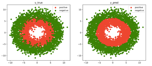
说明
笔记中很多代码案例来自于:
《20天吃掉那只Pytorch》
- github项目地址: https://github.com/lyhue1991/eat_pytorch_in_20_days
《30天吃掉那只TensorFlow2》
- github项目地址: https://github.com/lyhue1991/eat_tensorflow2_in_30_days
感兴趣的同学可以进入学习。
===========================================================================
我的笔记一部分是将这两项目中内容整理归纳,一部分是相应功能的内容自己找资料整理归纳。
笔记以MD格式存入我的git仓库,另外代码案例所需要数据集文件也在其中:可以clone下来学习使用。
《pytorch-tensorflow对比学习笔记》
github项目地址: https://github.com/Boris-2021/pytorch-tensorflow-Comparative-study
===========================================================================
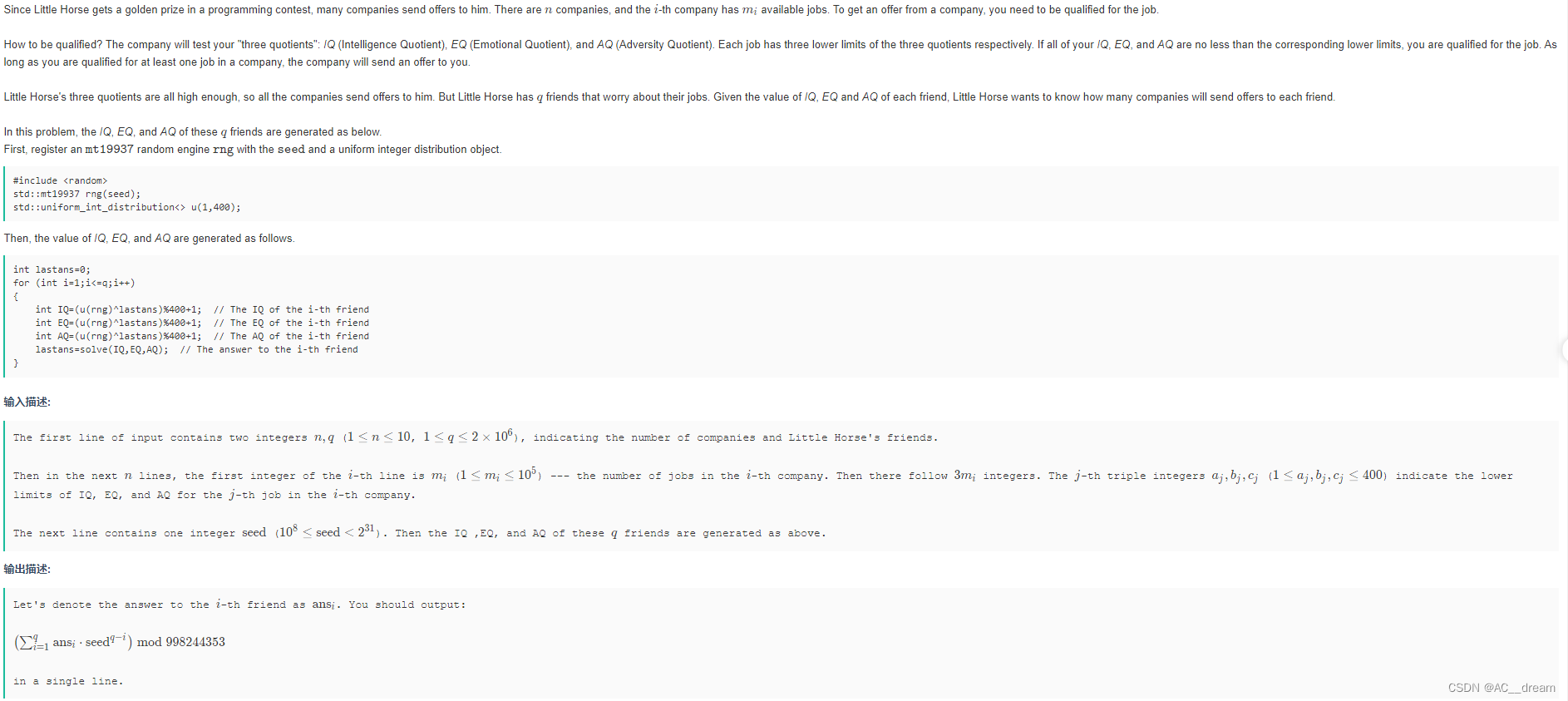
笔记中增加了很多趣味性的图片,增加阅读乐趣。
===========================================================================
感觉对你的学习有帮助,就点个星,点个赞,点个关注再走把,整理不易,拒绝白嫖从我做起!
边栏推荐
- (2022 Niu Ke Duo School IV) N-Particle Arts (Thinking)
- 25. Have you been asked these three common interview questions?
- TIM登陆时提示00001(TIM00001)
- typescript27-枚举类型呢
- 力扣(LeetCode)212. 单词搜索 II(2022.07.31)
- 解决ffmpeg使用screen-capture-recorder录屏,有屏幕缩放的情况下录不全的问题
- SQL Analysis of ShardingSphere
- (2022 Nioke Duo School IV) H-Wall Builder II (Thinking)
- typescript24 - type inference
- The Principle Of Percona Toolkit Nibble Algorithm
猜你喜欢

Dry goods!How to Construct SRv6-TE Performance Test Environment Using Instrumentation
(2022 Nioke Duo School IV) D-Jobs (Easy Version) (3D prefix or)

state compressed dp
干货!如何使用仪表构造SRv6-TE性能测试环境
(2022牛客多校四)D-Jobs (Easy Version)(三维前缀或)
状态压缩dp
Passive anti-islanding-UVP/OVP and UFP/OFP passive anti-islanding model simulation based on simulink

The difference between scheduleWithFixedDelay and scheduleAtFixedRate
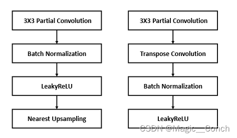
Progressive Reconstruction of Visual Structure for Image Inpainting 论文笔记
Code Interview Guide for Programmers CD15 Generating an Array of Windowed Maximums
随机推荐
(Codeforce 757) E. Bash Plays with Functions
LeetCode 27. 移除元素
The Principle Of Percona Toolkit Nibble Algorithm
Simulation of Active anti-islanding-AFD Active Anti-islanding Model Based on Simulink
Asynchronous reading and writing of files
怀念故乡的面条
微软 Win10 照片磁贴后的又一“刺客”,谷歌 Chrome 浏览器将在新标签页展示用户照片
开源许可证 GPL、BSD、MIT、Mozilla、Apache和LGPL的区别
请问shake数据库中想把源的db0的数据同步到目的db5,参数怎么设置呢?
剑指 Offer 68 - II. 二叉树的最近公共祖先
PMP 项目沟通管理
lambda
Invalid classes inferred from unique values of `y`. Expected: [0 1 2], got [1 2 3]
MySQL实践总结-
LeetCode 1189. “气球” 的最大数量
怀念故乡的月亮
typescript25 - type assertion
【云原生之kubernetes实战】kubernetes集群的检测工具——popeye
PMP 项目资源管理
Lawyer Interpretation | Guns or Roses?Talking about Metaverse Interoperability from the Battle of Big Manufacturers