Graphacademy course explanation: Fundamentals of neo4j graph data science

Last time I introduced GraphAcademy Inside to data scientists 、 Courses for data workers 《Neo4j Figure introduction to data science 》, From there we learned Neo4j GDS Basic concepts of 、 Install and enable , And the specific operation of graph projection .

Today, I will introduce the follow-up courses to you 《Neo4j Figure fundamentals of data science 》, Let's take a closer look at Neo4j GDS Provided graph algorithms and their applicable scenarios , And the basic usage of graph machine learning .

I hope I can understand the course content through reading this article , It is highly recommended to register for the course to start your own learning and to conduct actual coding and testing .

What is? GraphAcademy

Neo4j GraphAcademy yes Neo4j Launched an online interactive learning platform , Free of charge 、 Free to master the progress of online hands-on experimental training courses . Whether you're a developer 、 Operation and maintenance administrator , Or data scientists or engaged in machine learning 、 Artificial intelligence related personnel , Can be in GraphAcademy Find the right course for you .

All courses are conducted by Neo4j Professionals develop . Our goal is to provide you with enjoyable practical training , It contains text 、 Video and code challenges .

Each course you pass will unlock a badge , Share with friends and colleagues through your career profile or social network . By completing Neo4j Certification examination , You will unlock the limited edition Neo4j T T-shirt reward , And more importantly , Obtain the certificate of professional technology of graphic technology , This honor can be shown to employers and colleagues .

《Neo4j Figure fundamentals of data science 》 Course list

In this course , We will introduce data scientists to use Neo4j Graphic data science library (GDS) High level concepts that need to be understood when analyzing , The course covers GDS Graph algorithms and machine learning operations available in , And an example is given to illustrate how to use them on real data . The course continues to run in Neo4j The sandbox Of movie recommendations Data sets , You will use it throughout the course .

This course requires you to have some basic knowledge of graph data science and graph database . If not done 《Neo4j Figure introduction to data science 》 Course , It is recommended that you complete this course before proceeding to it .

Through this course, you will master ：

• Figure the execution mode of the algorithm
• Different categories of graph algorithms and common use cases
• How to be in GDS Running the native graph machine learning pipeline in

This course is divided into two sections , The outline of the catalogue is as follows ：

Graph algorithm

• Algorithm layer and execution mode
• Centrality and importance
• Challenge ： Centrality
• Find the way
• Challenge ： Find the shortest path
• Community testing
• Node embedding
• be similar

Figure machine learning

• An overview of machine learning
• Node classification pipeline
• Link prediction

Now come and have a look with me .

Graph algorithm

Figure algorithm product level and execution mode

Let's start with a piece of pseudo code ：

CALL gds[.<tier>].<algorithm>.<execution-mode>[.<estimate>](
	graphName: STRING,
	configuration: MAP
)

This code means to call Neo4j GDS library ,[] Said the optional ,<> Indicates that different values can be selected .

Figure algorithm product level

tier Express Neo4j GDS Different levels of products ：alpha、beta and Official version .

• Alpha： Indicates that the algorithm is in the experimental stage , It can be used for testing and verification , However, changes may occur as the version is updated . You need to specify the tier The value of is alpha To call Alpha Version of the algorithm .
• Beta： Indicates that the algorithm has gone through Alpha Version verification , It can be used as a candidate for the official version . You need to specify the tier by beta To call .
• Official version （production-quality）： I.e. production ready version , It indicates that the algorithm has passed the stability and scalability test , It can be used in a formal environment . Don't specify tier The default value of is to use the official version .

Execution mode

execution-mode Yes 4 Kind of , Used to specify how to handle the results of the algorithm ：

1. stream： Return the result of the algorithm as a record stream .
2. stats： Returns a single record of summary statistics , But don't write Neo4j Database or modify any data .
3. mutate： Write the result of the algorithm into the graph projection in memory and return a single record of summary statistics .
4. write： Write the result of the algorithm back to Neo4j Database and return a single record of summary statistics .

Memory estimate

estimate It is used to estimate the memory size required to execute an algorithm , from GDS Provide an estimation program to calculate .

Let's take a closer look at Neo4j GDS Algorithm provided , namely algorithm.

Centrality and importance

The centrality algorithm is used to determine the importance of different nodes in the graph , Common use cases include ：

• Recommendation system ： Identify and recommend the most influential or popular items in your content or product catalog
• Supply chain analysis ： Find the most critical node in the supply chain , Whether it's a supplier in the network 、 Raw materials in finished products or ports in the route
• Fraud and anomaly detection ： Find users who have many shared identifiers or act as bridges between many communities

Degree centrality algorithm

Degree centrality is one of the most common and simplest centrality algorithms . It calculates the number of relationships a node has （ Degrees ）. stay GDS In the implementation , We specially calculate The degree of Centrality , That is, the count of outgoing relationships from nodes . such as ：

//get top 5 most prolific actors (those in the most movies)
//using degree centrality which counts number of `ACTED_IN` relationships
CALL gds.degree.stream('proj')
YIELD nodeId, score
RETURN gds.util.asNode(nodeId).name AS actorName, score AS numberOfMoviesActedIn
ORDER BY numberOfMoviesActedIn DESCENDING, actorName LIMIT 5

PageRank Algorithm

Another common centrality algorithm is PageRank, Used to measure the influence of nodes in a directed graph , Especially when relationships imply some form of movement flow Under the circumstances , For example, payment network 、 Supply chain and logistics 、 signal communication 、 Route and website and link graph .PageRank The importance of nodes is estimated by calculating the number of incoming relationships from adjacent nodes , The weight of these neighboring nodes is the importance and out of degree centrality of these neighbors . The basic assumption is , More important nodes may have proportionally more incoming relationships from other import nodes .

If you are interested in further research , our PageRank Documentation will provide information about PageRank A comprehensive technical explanation of .

Other centrality algorithms

• Intermediary centrality ： Measure the degree to which a node is among other nodes in the graph . It is usually used to find nodes that serve as bridges from one part of a subgraph to another .
• Centrality of eigenvectors ： Measuring the transmission effects of nodes . Be similar to PageRank, But it only applies to the largest eigenvector of adjacency matrix , So it doesn't converge in the same way , And tend to prefer height nodes more strongly . It may be more appropriate in some use cases , Especially those use cases with undirected relationships .
• ArticleRank：PageRank A variant of , It assumes that relationships from low degree nodes have a higher impact than those from high degree nodes .

Can be in GDS The central part of the document Find a complete list of centrality algorithms for all product layers .

Challenge ： Degree centered practice

If the page doesn't pop up Neo4j Browser window , You can click the first button in the lower right corner to switch . I hope you can pass , Remember GDS The process of ？ First do the projection and then execute the algorithm .

Path finding

The path finding algorithm finds the shortest path between two or more nodes or evaluates the availability and quality of the path . Common use cases are ：

• Supply chain analysis ： Determine the fastest route between origin and destination or between raw materials and finished products
• Customer journey ： Analyze the events that make up the customer experience . for example , In the field of health care , This can be the experience of inpatients from admission to discharge

Dijkstra Source - Target shortest path

A common industry standard similarity algorithm is Dijkstra. It calculates the shortest path between the source node and the target node . And GDS Like many other path finding algorithms in ,Dijkstra Support weighting relationships when comparing paths to take into account distance or other cost attributes .

Here's how to use Dijkstra Source - Target the shortest path to find actors “Kevin Bacon” and “Denzel Washington” An example of the shortest path between .

MATCH (a:Actor)
WHERE a.name IN ['Kevin Bacon', 'Denzel Washington']
WITH collect(id(a)) AS nodeIds
CALL gds.shortestPath.dijkstra.stream('proj', {sourceNode:nodeIds[0], TargetNode:nodeIds[1]})
YIELD sourceNode, targetNode, path
RETURN gds.util.asNode(sourceNode).name AS sourceNodeName,
    gds.util.asNode(targetNode).name AS targetNodeName,
    nodes(path) as path;

Other routing algorithms

other GDS Production layer path finding algorithms can be divided into the following sub categories ：

Two The shortest path between nodes ：

• A* Shortest path ： Dijkstra An extension of , It uses heuristic functions to speed up computation .
• Yen Shortest path ：Dijkstra An extension of , You can find multiple top k Shortest path .

The shortest path between a source node and multiple other target nodes ：

• Dijkstra Single source shortest path ：Dijkstra Realize the shortest path between one source and multiple targets .
• Incremental step single source shortest path ： Parallelized shortest path computation . Than Dijkstra Single source shortest path calculation is faster , But use more memory .

General path search between a source node and multiple other target nodes ：

• Breadth first search ： In each iteration, the path is searched in the order of increasing distance from the source node .
• Depth-first search ： Search along a single multi hop path as much as possible in each iteration .

Can be in Path lookup document Find a complete list of central algorithms across all product tiers in .

Challenge ： Look for the shortest path

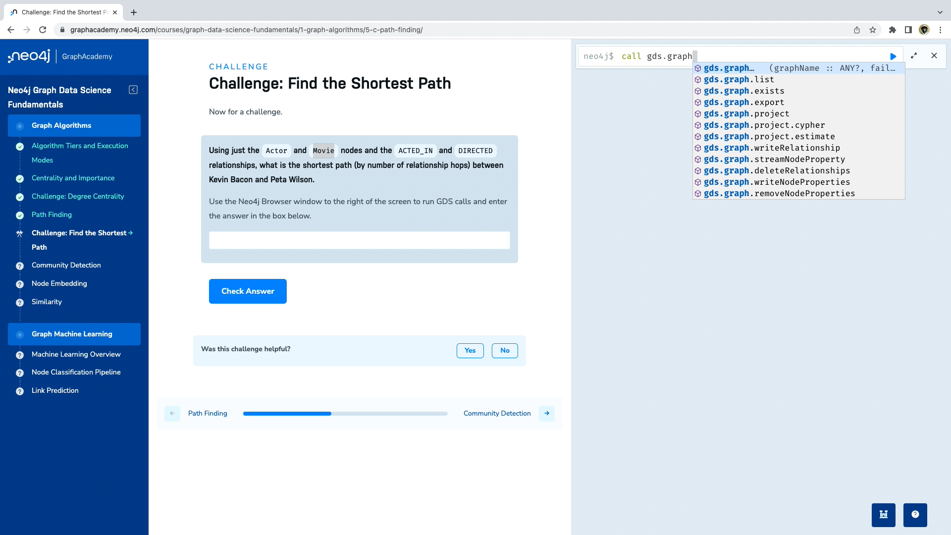
Again , You can Neo4j Browser Force to execute arbitrary queries . I hope you can pass .

Community testing

The community detection algorithm is used to evaluate the clustering or partitioning of node groups in the graph .GDS Most of the community detection functions in focus on distinguishing these node groups and assigning them ID, Conduct downstream analysis 、 Visualization or other processing . Common use cases include ：

• Fraud detection ： By identifying suspicious transactions and / Or accounts that share identifiers with each other to discover fraud circles .
• Customer 360： Disambiguate multiple records and interactions into one customer profile , In this way, the organization can provide a summary source of facts for each customer .
• Market segmentation ： By priority 、 Behavior 、 Interest and other criteria divide the target market into accessible subgroups .

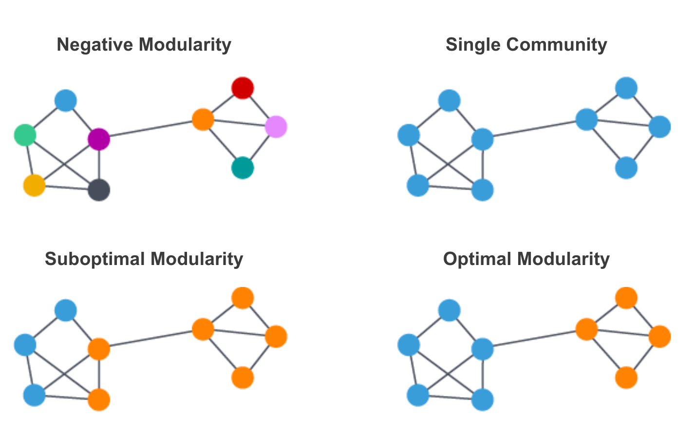
Louvain Community testing

A common community detection algorithm is Louvain.Louvain Maximize modular scores for each community , Modularity quantifies the quality of assigning nodes to communities . This means that the connection density of nodes in the evaluation community is compared with the connection degree of nodes in the random network .

Louvain Hierarchical clustering method is used to optimize this modularization , This method recursively merges communities together . There are several parameters that can be adjusted Louvain To control its performance and the number and size of the communities it generates . This includes the maximum number of iterations and level of hierarchy to be used, as well as for evaluating convergence / Tolerance parameter of stop condition . our Louvain file These parameters and adjustments are described in more detail .

Other community detection algorithms

Here are some other production level community detection algorithms . Sure Check the algorithm document in the community Find a complete list of all community detection algorithms in .

• Tag spread ： And Louvain Similar intent . A fast algorithm with good parallelization . Great for large charts .
• Weakly connected components （WCC）： Divide the graph into connected node sets , bring
  1. Each node can be accessed from any other node in the same collection
  2. There is no path between nodes of different sets
• Triangle count ： Calculate the number of triangles per node . It can be used to test the cohesion of the community and the stability of the map .
• Local clustering coefficient ： Calculate the local clustering coefficient of each node in the graph , This is an indicator of how nodes cluster with their neighbors .

Node embedding

The goal of node embedding is to compute the low dimensional vector representation of nodes , Make the similarity between vectors （ For example, dot product ） Similar to the similarity between nodes in the original graph . These vectors , Also known as embedding , For exploratory data analysis 、 Similarity measurement and machine learning are very useful .

The following figure illustrates the concept behind node embedding , That is, the nodes that are close in the graph will finally be close in the two-dimensional embedded space . therefore , Embed get structure from graph , namely n Dimension adjacency matrix , It is approximated as a two-dimensional vector of each node . Because the dimensions are significantly reduced , Embedded vectors are more efficient in the downstream process . for example , They can be used for cluster analysis , Or as a feature of training node classification or link prediction model .

The node embedding vector itself does not provide insight , They are created to enable or extend other analytics . Common workflows include ：

• Exploratory data analysis (EDA), For example, visualization TSNE Embeddedness in the diagram , To better understand the graph structure and potential node clusters
• Similarity measurement ： Node embedding allows you to use K Nearest neighbor (KNN) Or other techniques to extend similarity inference in large graphs . This is useful for extending memory based recommendation systems , For example, the variation of collaborative filtering . It can also be used in the field of fraud detection semi supervised technology , for example , We may want to generate clues similar to a set of known fraudulent entities .
• The characteristics of machine learning ： Node embedding vectors are naturally inserted as features of various machine learning problems . for example , In the online retailer's user purchase chart , We can use embedding to train the machine learning model to predict the products that users may be interested in buying next .

FastRP

GDS Provides a custom implementation of node embedding technology , It is called fast random projection , Or for short FastRP.FastRP Using probability sampling technique to generate sparse representation of graph , So that we can Very quickly Calculate the embedding vector , Its quality is similar to that of traditional random walk and neural network technology （ Such as Node2vec and GraphSage） The resulting vector is quite . This makes FastRP Becoming begins in GDS Explore the best options for embedding charts in .

Other node embedding algorithms

GDS It's also achieved Node2Vec, It is based on the vector representation of random walk computing nodes in the graph , as well as GraphSage, It is an inductive modeling method that uses node attributes and graph structure to calculate node embeddedness .

Similarity degree

The similarity algorithm is used to infer the similarity between node pairs . stay GDS in , These algorithms run in batch on graph projection . When similar node pairs are identified according to the user specified metrics and thresholds , Draw a relationship with similarity score attributes between the pairs . According to the execution mode used when running the algorithm , These similarity relationships can stream transmission 、mutate To memory map or write Write back to the database . Common use cases include ：

• Fraud detection ： Discover potential fraudulent user accounts by analyzing the similarity between a set of new user accounts and tagged accounts .
• Recommendation system ： In online retail stores , Identify the item that matches the item that the user is currently viewing , To inform the impression and improve the purchase rate .
• Entity parsing ： Identify nodes that are similar to each other according to the activities or identification information in the diagram .

GDS There are two main similarity algorithms ：

• Node similarity ： The similarity between nodes is determined according to the relative proportion of shared adjacent nodes in the graph . Where explicability is important , Node similarity is a good choice , You can narrow the comparison to a subset of the data . Examples of downscaling include focusing only on a single community 、 Newly added nodes or nodes close to the subgraph of interest .
• K Nearest neighbor (KNN)： Determine the similarity according to the node attributes . If adjusted properly ,GDS KNN The implementation can be well extended to perform global reasoning on large graphs . It can be used in conjunction with embedding and other graph algorithms , According to the proximity in the figure 、 Node properties 、 Community structure 、 Importance / Centrality, etc. to determine the similarity between nodes .

Similar function

In addition to node similarity and KNN Out of algorithm ,GDS A set of functions is also provided , It can be used to calculate the similarity between two digital arrays using various similarity measures , Include jaccard、overlap、pearson、 Cosine similarity, etc . Full documentation will do stay Similarity Functions file Find . When you are interested in measuring the similarity between a single selection node pair at a time instead of calculating the similarity of the entire graph , These functions are very useful .

Figure machine learning

First, let's talk about GDS Why it helps to have a machine learning function , You can Neo4j Generate graph features in and export them to another environment for machine learning , for example Python、Apache Spark etc. . These external frameworks have great customization flexibility and adjust the machine learning model . however , You may wish to be in GDS There are many reasons for using graph based machine learning tools in ：

1. Manage complex model design ： Graph data is highly interconnected in nature , It brings complexity to the machine learning workflow , For those who are not familiar with graphs , These complexities can be difficult to capture and resolve . If not considered , These complexities can damage ML The validity of the model 、 Computational and predictive performance .GDS Pipelines include ways to address these complexities , Otherwise, these complexities are difficult to be generalized 、 Not graph specific ML Develop and maintain in the framework . The main example is the appropriate data splitting design 、 Deal with serious class imbalance and avoid data leakage in feature engineering .
2. Fast production path with strong database coupling ： because Neo4j Provided in GDS, So it's easy to put GDS ML Apply directly to Neo4j database . Once you're in GDS A pipe was trained in , The model will be automatically saved and deployed effectively —— Get ready to go through a simple predict Command pair from Neo4j The data of the database is used for prediction . Enterprise users can keep these models for reuse , They can also be published for sharing among teams .
3. Development and experiment ： Even for having mature and strong MLOps For experienced practitioners in the enterprise of workflow , Native ML Pipelines also eliminate many of the initial friction that is usually associated with graph machine learning . This allows you to experiment and test the model approach to get started quickly .

GDS Focus on end-to-end ML Workflow provides managed pipeline . Data selection 、 Feature Engineering 、 Data splitting 、 Superparametric configuration and training steps are coupled together in the pipe object , To track the required end-to-end steps . There are currently two supported ML Pipe type ：

• Node classification pipeline ： Supervised binary and multiclass classification of nodes
• Link prediction pipeline ： Whether there should be a relationship or... Between pairs of nodes “ link ” Monitoring forecasts for

These pipes have a train Program , Once the run , A trained model object will be generated . In turn, , These trained model objects have predict A process that can be used to predict data . You can go to GDS Has multiple pipes and model objects at the same time . Both pipes and models have a directory , Allows you to manage them by name , Similar to the graph projection in the graph directory .

Node classification pipeline

Here is GDS Diagram of medium and high level node classification mode , From the projection map through various steps to the final registration model and predict the data .

In practice , Training steps 1-6 Will be automatically executed by the pipeline . You will only be responsible for providing them with configuration and super parameters . therefore , At a higher level , Your workflow will classify nodes as follows , The same is true for link prediction ：

1. Project drawings and configure piping （ Order doesn't matter ）.
2. Use the command to execute the pipeline train.
3. predict Use the command to predict on the projection map . if necessary , You can use the graph to write write The operation writes the forecast back to the database .

Link prediction

GDS Binary classifiers are currently available , The goal is 0-1 indicators ,0 Indicates no link ,1 Indicates that there is a link . This type of link prediction is very effective in Undirected Graphs , A type of relationship between nodes in which you can predict a single label , For example, social networks and entity resolution .

Here is GDS Illustration of medium and advanced link prediction mode , From the projection map through various steps to the final registration model and predict the data .

You will notice that some of the additional steps here are similar to the node classification and other common steps that may have been used in the past ML The pipeline is different . namely ,feature-input There is an additional set in the relationship split , Now before the node attribute and feature generation step . In short , This is to deal with data leakage , To calculate model characteristics using the relationships you want to predict . This situation will allow the model to use information from features that are not normally available , This leads to overly optimistic performance indicators . It can be found in the document Read more about data splitting methods in .

Figure two sections of machine learning have detailed example code , You can click “Run in Sandbox” On the current page Neo4j Browser See the implementation results in .

Course summary

Congratulations ！ You should now be ready to use Neo4j The graph data science library runs your first graph algorithm .

In the first module Graph algorithm in , You know Neo4j GDS Graph algorithms available in and how to use them on real data .

In the second module Figure machine learning in , You know GDS Native machine learning operations , Including node classification pipeline and link prediction .

next step

Now you are right Neo4j Graph data science GDS Library graph algorithm and machine learning have some basic understanding and practice , You can read GDS For details , Even visit GDS Source code to improve together . Now is the time to use it in real business GDS 了 , Please feel free to keep in touch with us .

The resources

The course address is ：https://graphacademy.neo4j.com/courses/graph-data-science-fundamentals/

《Neo4j Figure introduction to data science 》 Course ：https://graphacademy.neo4j.com/courses/gds-product-introduction/

Course data sets ：https://github.com/neo4j-graph-examples/recommendations