Shandong University machine learning experiment 5 SVM

Machine learning experiment of Shandong University 5 The report

Experimental hours ： 6 Date of experiment ：2021.11.20

Experimental topics — Experiment 5 : SVM

The experiment purpose

This exercise gives you practice with using SVMs for both linear and non-linear classification

Use SVM Linear and nonlinear classification

Experimental environment

Software environment

​ Windows 10 + Matlab R2020a

Experimental steps and contents

understand SVM

SVM The classification model can be described as the following model ：

But the above model has too many constraints , So we can change , Get the dual model .

Because the dual problem constraint is simple only one ${\alpha }_i>=0$ Constraints

Lagrange dual problem:

Karush-Kuhn-Tucher(KKT) Condition

KKT Conditions ： If the strong duality satisfies KKT Conditions :

1. stability

2. Primal feasibility:

3. Dual feasibility

   

4. Complementary relaxation :

   

Besides KKT The condition is a sufficient condition for strong duality , And we solve the dual problem by KKT Conditions to solve

Using kernel function and soft interval SVM Of Model Described below :

yes

Quadratic programming

In this experiment, we need to solve QP problem , It uses Matlab Provided quadprog function :

Kernel Methods Kernel function

The essence is to map the original data Or upgrade dimension .

It's usually a N Dimension becomes $N\ast (N-1)÷2$ dimension

[ Failed to transfer the external chain picture , The origin station may have anti-theft chain mechanism , It is suggested to save the pictures and upload them directly (img-F0HfSHPO-1637667157053)(C:/Users/12042/AppData/Roaming/Typora/typora-user-images/image-20211121201415845.png)]

Soft space SVM:

That is, some are allowed to be misclassified , But limit the number

Turn into

then ${\xi }_i$ yes slack variable Relax variables ( Similar to regular penalty term )

therefore model Turn into ：

C Balance margin as well as misclassification

such as small C: Then it means that you want a larger interval

​ large C: Indicates that you want less misclassification

The corresponding Lagrange function ：

Added a " r " Five parameters are required ：$\omega b\xi \alpha r$

adopt QP The problem is solved and $\alpha$

And then through duality + KKT obtain

---

Task 1: Linear SVM

Plot decision boundary of the SVM

First read in the data , Draw a scatter diagram ： Data set 1 is as follows ： It can be seen that there is an obvious linear boundary Boudary

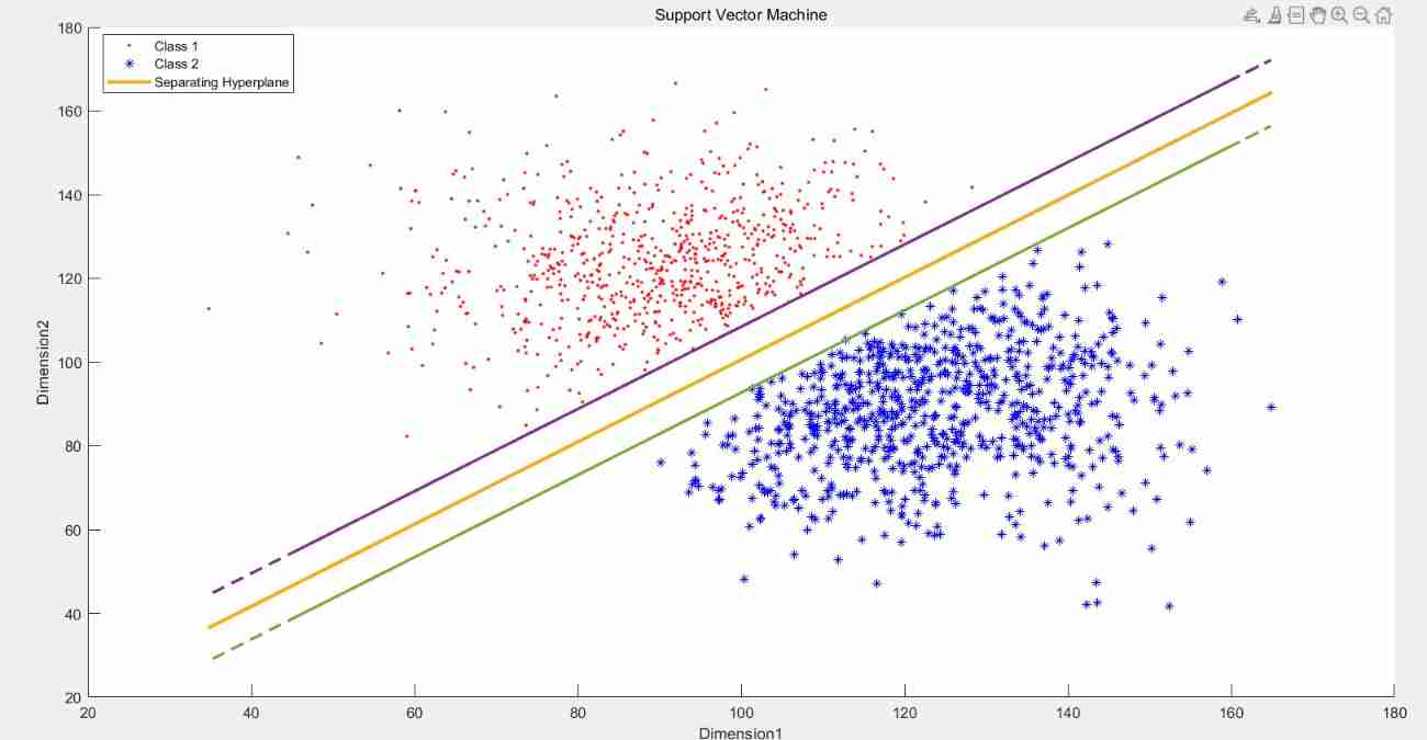
The following figure shows the data set II ： The decomposition interval is not as obvious as one, but it can still be seen that there is

Then use QP Problem solver :quadprog To solve the

obtain $\alpha$ Value

Here's the problem ：matlab There are some $\alpha$ The order of magnitude is about -18 Power , These are thought to be solved 0 Of , Do a process to get $\alpha$ Here are two pictures Namely data1data2 C In very large cases $\alpha$

Yes DataSet1 That is, if you select a larger C Less misclassification , Found Support Vector There are only three , In this way, only C drop to 0.016 Will begin to have a limiting effect

Yes DataSet12 That is, if you select a larger C Less misclassification , Found Support Vector There are only three , In this way, only C drop to 1.5 Will begin to have a limiting effect

So if you use a larger C To train DataSet1 The result is shown in the figure below , That is Hard Margin

So if you use a smaller C To train DataSet1 The result is shown in the figure below , That is Soft Margin, There are no misclassified points , But some fell on boundary Points within

Yes Dataset2 It's the same thing C large ：

Yes Dataset2 It's the same thing C More hours ：

Use the test data to evaluate the SVM classifier and show the fraction of test examples which were misclassified

First ： Two test data The performance of ： Accuracy = 100% Therefore, there is no misclassification , Draw the histogram of classification effect

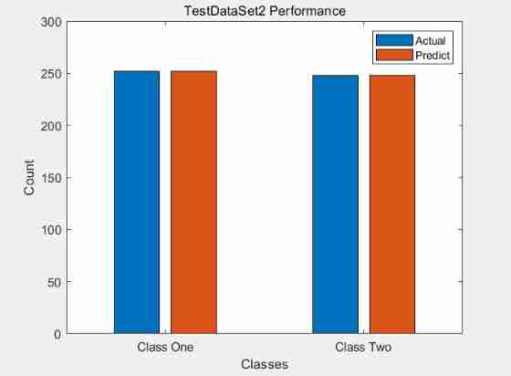
test Data Performance of ： You can see There is no misclassification ！

Try different values of the regularization term C, and report your observations.

Data one Set up C = 0.001 : 0.001 : 0.01

Test and find all score All are 100%

And then part of it boundary The picture is shown below

About DataSet2 Use C = 0.001 - 0.01

The accuracy is still 100% Don't show

Show only part of the situation

Task 2: Handwritten Digit Recognition（ Handwritten numeral recognition 0 & 1）

Preprocess Data

Processing data , For the given image Data for a simple process , Can get image In general ：

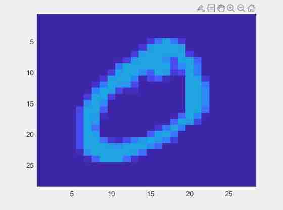
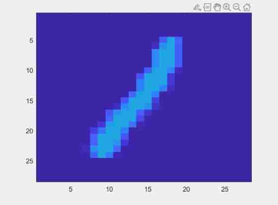
That is to say, it is drawn directly by using the gray value

Besides , This topic Image Tensor SIZE = 1 X 28 X 28 And then use extractLBPFeatures() to feature Conduct One Pooling + Flatten Get one 1X1X59 Of feature

Corresponding SVM There is 59 individual feature($X_i$) then Conduct train

Train Plain-vanilla SVM

Use 12000+ Picture data will appear

Because the data is too big Write QPsolver Of H Matrices are all 1w X 1w size Of It's too big ！ Maybe there is something wrong with your computer

therefore Reduce the following size Every random sampling is not repeated 1000 individual image Come on train

Returns the sampling data and the corresponding tag as well as the original set Position in

%%
function [sample_Datas,sample_labels,chose_set] = sample_random(num,datas,labels)
    % datas  For raw data  num  Is the target number 
    chose_set = [];%1000*1  Is this 1000 The number is the same set Medium id
    R = length(datas);
    a = rand(R,1);
    [b,c] = sort(a);
    chose_set = c(1:num,1);
    chose_set = sort(chose_set);
    sample_Datas = datas(chose_set,:);
    sample_labels = labels(chose_set,:);
end

After training Do not apply soft margin The accuracy obtained is probably **99.4%——99.5%** about

For example, once there were six misclassifications (Training Data Medium ) Their pictures are shown below ：

It can be seen clearly For example, in the middle ‘2’ Flat below 1 And the last one ‘6’ It is very likely that there is misclassification itself , They do not conform to 0 1 Of feature

---

To test :

Get accuracy = 98.58 23 Zhang image error Some are shown below

The possible reason is The writing is not standard It's not like 0 Neither 1 feature It's not obvious

Experiment with different values of the regularization term C

Pick 10 individual values

C = [0.01 0.05 0.1 0.5 1.5 3 5 7.5 10 15]; Training + test

Found in C=0.1 After that, the accuracy will reach 90% 了

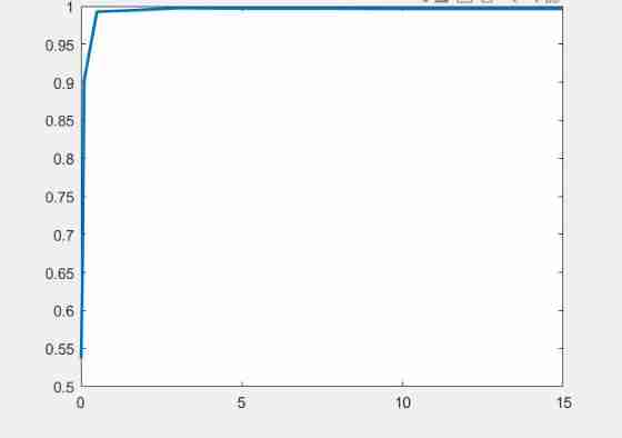
therefore More detailed points are as follows C = 0.02 : 0.02 : 0.2 give the result as follows ： Two tests were carried out Try to avoid the influence of random sampling

namely Larger C signify Less misclassfication and Higher Accuracy

What value of C gives you the best training error on the dataset from part? & How does the test error for this choice of C compare with the test error you computed in part (i)?

sampling 25 individual C Training , The training error and the corresponding test error are obtained

When C = 2 when ,train When the effect is the best 0.9900, But when C=1.8 when ,test The best effect is 0.9957

All in all C The bigger it is , There may be over fitting , Lead to in train The effect becomes better , however test Upward variation

Task 3: Non-Linear SVM

Plot the Data

It is found that there is no obvious linear dividing line

So you need to use a kernel Upgrade the dimension , We expect the data to have a linearly separable hyperplane in high dimensional space

RBF kernel

The Gaussian kernel function

Writing in this experiment ：

Model writing at this time ：

Use RBF kernel To test ;

$\gamma =[1;10;100;1000]$

It can be found that with $\gamma$ increase Although the classification effect is getting better But gradually classification over fitting

Task 4: Use SMO Instead Of QP solvers

Write a suggested SMO Algorithm instead of solving large-scale problems QP problem

Input: data 、 label 、 Parameters bias And the maximum number of iterations and tolerance values

Algorithm: Every iteration

​ Choose two according to the rules $\alpha$

​ Keep other Lagrange multipliers constant , to update ${\alpha }_1{\alpha }_2$

output: $\alpha bias$

Wrote a simplified version of SMO Algorithm

Traverse to select one ${\alpha }_1$ Then pick one at random ${\alpha }_2$ But this ${\alpha }_2$ Conditions must be met ：

Conclusion analysis and experience

• Different values Of C

  In the first two datasets , Different C It has no effect on the final accuracy , All are 100%, It shows that there is a linearly separable hyperplane in both data sets . however C For the decided boundary The scope of is influential ,C The smaller it is , As a result, the penalty item weight becomes smaller , Will lead to a bigger margin, But there may be more misclassification .

• Different values Of C in Handwritten Digit Recognition

  In handwritten numeral recognition , as long as C More than a certain value , for example 0.1, After that, the accuracy can be stabilized at 99% about , In my experimental tests ,C=2 yes train The highest accuracy 99%,C=1.8 when ,test The best effect is 0.9957

  All in all C The bigger it is , There may be over fitting , Lead to in train The effect becomes better , however test Upward variation

• $\gamma$ stay Nonlinear SVM Influence

  With $\gamma$ Increase will gradually over fit , So balance is needed $\gamma$

• Kernel function

  In this experiment RBF kernel The Gaussian kernel function , Note that using kernel functions does not require computation $\varphi$ Just calculate matrix K that will do

• SMO

  SMO It is to transform a large quadratic program into several small quadratic programs

  for i=1:iter

  ​ a. According to preset rules , Select two from all samples

  ​ b. Keep other Lagrange multipliers constant , Update the Lagrange multiplier corresponding to the selected sample

  end

  How to update $\alpha 1\alpha 2$ Well ？

Random selection for simplification , So the effect is average

Maybe the training times are too few , Although this dividing line is quite unreasonable , But the accuracy can also be 73.6%

See the code at the end

Experiment source code

Lab51.m：

%%  Experiment five  SVM  Support vector machine 
%%  Soft space 
%%  Reading data   Draw a scatter diagram 
clear,clc;
Trainning_Datas = load('training_1.txt');
Data_x1 = Trainning_Datas(:,1);
Data_x2 = Trainning_Datas(:,2);
Data_label = Trainning_Datas(:,3);
X = [Data_x1,Data_x2];
Y = Data_label;
% scatter(Data_x1,Data_x2,'.','b');

%%  utilize quadprog  solve  $\alpha$
%  seek Min 1/2 yax - a
% The objective function must be written in a quadratic form H The form of adding to a matrix 
% Cs = 0.001:0.001:0.01; %  Hyperparametric 
% for num = 1 : 10
    H=[];% Objective function H
    C = 0.006;
    for i=1:length(X)% All samples must be traversed 
        for j=1:length(X)
            H(i,j)=X(i,:)*(X(j,:))'*Y(i)*Y(j);
        end
    end
    F = -1 * ones(length(X),1);% Objective function F

    % Equality constraints 
    aeq=Y';
    beq=zeros(1,1);
    % Inequality constraints   No, 
    ub=[];
    ib=[];
    % Independent variable constraint 
    lb = zeros(length(X),1);% Lower bound 
    ub = zeros(length(X),1);% upper bound 
    ub(:,:) = C;
    %  solve alpha
    [alpha,fval]=quadprog(H,F,[],[],aeq,beq,lb,ub);% Second planning problem 

    %%  Will find out a lot alpha Very close to 0  That's not support vector
    %  however   How many points are appropriate ？？  About three   Because the dividing line is still very clear 
    % BUT  Soft interval shall be fully calculated  so  There is no need to divide 
    %  Be careful ！！ data1  Obviously no need for soft spacing   All without misclassification ！( Unless C Very small ~)
    %  It's normal. It's probably 0.01  Just in the early days 
    plot(alpha,'b') % obvious 
    title('\alpha of QP')
    xlabel('x')
    ylabel('\alpha')
    a = alpha;
    %  Or choose to deal with   Because normally there are =0 Of 
    for i=1:length(a)
        if a(i)<1e-8
            a(i)=0;
        end
    end
    %%  seek w
    W = 0; %  coefficient matrix 
    u = 0;
    j = find(a > 0 & a < C);
    for i = 1:length(X)
            W = W + a(i)*Y(i)*X(i,:)';
    end

    %%  seek r
    R = 0;
    R = C - a;

    %%  seek B  Is to use the support vector
    %  A bit of a problem. ...  Namely   Only S V  Or use it all 
    %  Formula is S V  however   Calculate the SV  and   Ideal SV Dissimilarity 
    j = find(a > 0 & a < C); % look for  S V
    nums = length(j); %  How many? 
    temp = Y - X*W;
    B = sum(temp(j)) / nums;

    %%  Draw Boundary
    k = -W(1)./W(2);
    bb = -B./W(2);

    group1 = find(Data_label==1);
    group2 = find(Data_label==-1);
    scatter(Data_x1(group1),Data_x2(group1),'.','r');
    hold on
    scatter(Data_x1(group2),Data_x2(group2),'*','b');
    hold on

    yy = k.*Data_x1 + bb;
    plot(Data_x1,yy,'-','LineWidth',2.5)
    hold on
    yy = k.*Data_x1 + bb + 1./W(2);
    plot(Data_x1,yy,'--','LineWidth',2)
    hold on
    yy = k.*Data_x1 + bb - 1./W(2);
    plot(Data_x1,yy,'--','LineWidth',2)
    title('Support Vector Machine C = 0.006')
    xlabel('Dimension1')
    ylabel('Dimension2')
    legend('Class 1','Class 2','Separating Hyperplane')

    %% Test
    Predict = [];
    Test_Datas = load('test_1.txt');
    test_x1 = Test_Datas(:,1);
    test_x2 = Test_Datas(:,2);
    test_X = [test_x1,test_x2];
    test_Y = Test_Datas(:,3);
    Predict = sign(test_X*W + B);
    Judge=(Predict==test_Y);
    score = sum(Judge)./length(test_X)

    %%  Draw Bar on testdata
    test_Class1_nums = length(find(test_Y==1));
    test_Class2_nums = length(find(test_Y==-1));
    Predict_Class1_nums = length(find(Predict==1));
    Predict_Class2_nums = length(find(Predict==-1));
    Bar_y = [test_Class1_nums,Predict_Class1_nums;test_Class2_nums,Predict_Class2_nums];
    Bar_x = categorical({'Class One','Class Two'});
    bar(Bar_x,Bar_y)
    legend('Actual','Predict');
    xlabel('Classes');
    ylabel('Count');
    title(['TestDataSet1 Performance']);

Lab52.m

%%  Experiment five  SVM  Support vector machine 
%%  Soft space 
%%  Reading data   Draw a scatter diagram 
clear,clc;
Trainning_Datas = load('training_2.txt');

Data_x1 = Trainning_Datas(:,1);
Data_x2 = Trainning_Datas(:,2);
Data_label = Trainning_Datas(:,3);
X = [Data_x1,Data_x2];
Y = Data_label;
%scatter(Data_x1,Data_x2,'.','r');

%%  utilize quadprog  solve  $\alpha$
%  seek Min 1/2 yax - a
% The objective function must be written in a quadratic form H The form of adding to a matrix 
C = 1; %  Hyperparametric 
H=[];% Objective function H
for i=1:length(X)% All samples must be traversed 
    for j=1:length(X)
        H(i,j)=X(i,:)*(X(j,:))'*Y(i)*Y(j);
    end
end
F = -1 * ones(length(X),1);% Objective function F
% Equality constraints 
aeq=Y';
beq=zeros(1,1);
% Inequality constraints   No, 
ub=[];
ib=[];
% Independent variable constraint 
lb = zeros(length(X),1);% Lower bound 
ub = zeros(length(X),1);% upper bound 
ub(:,:) = C;
%  solve alpha
[alpha,fval]=quadprog(H,F,[],[],aeq,beq,lb,ub);% Second planning problem 

%%  Will find out a lot alpha Very close to 0  That's not support vector
%  however   How many points are appropriate ？？  About three   Because the dividing line is still very clear 
% BUT  Soft interval shall be fully calculated  so  There is no need to divide 
%  Be careful ！！ data1  Obviously no need for soft spacing   All without misclassification ！( Unless C Very small ~)
%  It's normal. It's probably 0.01  Just in the early days 
plot(alpha,'b') % obvious 
title('\alpha of QP')
xlabel('x')
ylabel('\alpha')
a = alpha;
%  Or choose to deal with   Because normally there are =0 Of 
for i=1:length(a)
    if a(i)<1e-8
        a(i)=0;
    end
end
%%  seek w
W = 0; %  coefficient matrix 
u = 0;
j = find(a > 0 & a < C);
for i = 1:length(X)
        W = W + a(i)*Y(i)*X(i,:)';
end

%%  seek r
R = 0;
R = C - a;

%%  seek B  Is to use the support vector
%  A bit of a problem. ...  Namely   Only S V  Or use it all 
%  Formula is S V  however   Calculate the SV  and   Ideal SV Dissimilarity 
j = find(a > 0 & a < C); % look for  S V
nums = length(j); %  How many? 
temp = Y - X*W;
B = sum(temp(j)) / nums;

%%  Draw Boundary
k = -W(1)./W(2);
bb = -B./W(2);
figure
group1 = find(Data_label==1);
group2 = find(Data_label==-1);
scatter(Data_x1(group1),Data_x2(group1),'.','r');
hold on
scatter(Data_x1(group2),Data_x2(group2),'*','b');
hold on


yy = k.*Data_x1 + bb;
plot(Data_x1,yy,'-','LineWidth',0.5)
hold on
yy = k.*Data_x1 + bb + 1./W(2);
plot(Data_x1,yy,'--','LineWidth',1)
hold on
yy = k.*Data_x1 + bb - 1./W(2);
plot(Data_x1,yy,'--','LineWidth',0.5)
title('Support Vector Machine C = 1')
xlabel('Dimension1')
ylabel('Dimension2')
legend('Class 1','Class 2','Separating Hyperplane')

%% Test
Predict = [];
Test_Datas = load('test_2.txt');
test_x1 = Test_Datas(:,1);
test_x2 = Test_Datas(:,2);
test_X = [test_x1,test_x2];
test_Y = Test_Datas(:,3);
Predict = sign(test_X*W + B);
Judge=(Predict==test_Y);
score = sum(Judge)./length(test_X)

%%  Draw Bar on testdata
figure
test_Class1_nums = length(find(test_Y==1));
test_Class2_nums = length(find(test_Y==-1));
Predict_Class1_nums = length(find(Predict==1));
Predict_Class2_nums = length(find(Predict==-1));
Bar_y = [test_Class1_nums,Predict_Class1_nums;test_Class2_nums,Predict_Class2_nums];
Bar_x = categorical({'Class One','Class Two'});
bar(Bar_x,Bar_y)
legend('Actual','Predict');
xlabel('Classes');
ylabel('Count');
title(['TestDataSet2 Performance']);

Lab53.m

%% Hand
clc,clear;
%  Save one map  this 1000 individual sampledata Inside   Corresponding to the original number 
[Train_Data_X,Train_Labels] = strimage();
[Train_Data_X,Train_Labels,Map_id] = sample_random(1000,Train_Data_X,Train_Labels);

%Size = 12665 * 59
%% 
Cs = 0.02:0.02:0.2;
for Cnum=1:10
C = Cs(Cnum); %  Hyperparametric 
H=[];% Objective function H
for i=1:length(Train_Data_X)% All samples must be traversed 
    for j=1:length(Train_Data_X)
        H(i,j)=Train_Data_X(i,:)*(Train_Data_X(j,:))'*Train_Labels(i)*Train_Labels(j);
    end
end
F = -1 * ones(length(Train_Data_X),1);% Objective function F
%% 
% Equality constraints 
aeq=Train_Labels';
beq=zeros(1,1);
% Inequality constraints   No, 
ub=[];
ib=[];
% Independent variable constraint 
lb = zeros(length(Train_Data_X),1);% Lower bound 
ub = [];% There is no upper bound requirement 
ub = zeros(length(Train_Data_X),1);% upper bound 
ub(:,:) = C;
%  solve alpha
[alpha,fval]=quadprog(H,F,[],[],aeq,beq,lb,ub);% Second planning problem 

%%
% plot(alpha,'b') % obvious 
% title('\alpha of QP')
% xlabel('x')
% ylabel('\alpha')
a = alpha;
%  Or choose to deal with   Because normally there are =0 Of 
for i=1:length(a)
    if a(i)<1e-8
        a(i)=0;
    end
end

%%  seek W
W = 0; %  coefficient matrix 
u = 0;
j = find(a > 0);
for i = 1:length(Train_Data_X)
        W = W + a(i)*Train_Labels(i)*Train_Data_X(i,:)';
end
%% 
j = find(a > 0); % look for  S V
nums = length(j); %  How many? 
temp = Train_Labels - Train_Data_X*W;
B = sum(temp(j)) / nums;
%% 
% Predict = [];
% test_X = Train_Data_X;
% test_Y = Train_Labels;
% Predict = sign(test_X*W + B);
% Judge=(Predict==test_Y);
% score = sum(Judge)./length(test_X)
%%  Look for misclassified 
% misclass =[];
% misclass = find(Judge==0)
% for i=1:length(misclass)
%     id = misclass(i);
%     ori_id = Map_id(id);
%     showimage(ori_id)
% end
%% Test
[Test_Data_X,Test_Labels] = strimagetest();
Predict = [];
test_X = Test_Data_X;
test_Y = Test_Labels;
Predict = sign(test_X*W + B);
Judge=(Predict==test_Y);
score(Cnum) = sum(Judge)./length(test_X)
%%  Look for misclassified 
% misclass =[];
% misclass = find(Judge==0)
% for i=1:length(misclass)
%     id = misclass(i);
%     ori_id = Map_id(id);
%     showimage(ori_id)
% end
end
figure
plot(Cs,score,'LineWidth',2)
title('Performance in Different C')
xlabel('C')
ylabel('Accuracy')
ylim([0.5 1])
axis()
%%
function [sample_Datas,sample_labels,chose_set] = sample_random(num,datas,labels)
    % datas  For raw data  num  Is the target number 
    chose_set = [];%1000*1  Is this 1000 The number is the same set Medium id
    R = length(datas);
    a = rand(R,1);
    [b,c] = sort(a);
    chose_set = c(1:num,1);
    chose_set = sort(chose_set);
    sample_Datas = datas(chose_set,:);
    sample_labels = labels(chose_set,:);
end

Revised strimage.m

function [AllPic_Feature,All_Labels] = strimage()
  fidin = fopen('train-01-images.svm'); %  open test2.txt file  
  j = 1;
  apres = [];
   AllPic_Feature = [];
   All_Labels=[];
while ~feof(fidin)
  tline = fgetl(fidin); %  Read line from file  
  apres{j} = tline;
  %  Process this line 
  a = char(apres(j));
  All_Labels = [All_Labels;str2num(a(1:2))];
  lena = size(a);
  lena = lena(2);
  xy = sscanf(a(4:lena), '%d:%d');
  lenxy = size(xy);
  lenxy = lenxy(1);
  grid = [];
  grid(784) = 0;
  for i=2:2:lenxy  %%  One number apart 
      if(xy(i)<=0)
          break
      end
    grid(xy(i-1)) = xy(i) * 100/255;
  end
  grid1 = reshape(grid,28,28);
  grid1 = fliplr(diag(ones(28,1)))*grid1;
  grid1 = rot90(grid1,3);
  image_f = extractLBPFeatures(grid1);
  AllPic_Feature = [AllPic_Feature;image_f];
  
  j = j+1;
end

end

showimage.m:

function showimage(n)
  fidin = fopen('train-01-images.svm'); %  open test2.txt file  
  i = 1;
  apres = [];

while ~feof(fidin)
  tline = fgetl(fidin); %  Read line from file  
  apres{i} = tline;
  i = i+1;
end

  a = char(apres(n));
  
  lena = size(a);
  lena = lena(2);
  xy = sscanf(a(4:lena), '%d:%d');

  lenxy = size(xy);
  lenxy = lenxy(1);
  
  
  grid = [];
  grid(784) = 0;
  for i=2:2:lenxy  %%  One number apart 
      if(xy(i)<=0)
          break
      end
    grid(xy(i-1)) = xy(i) * 100/255;
  end
  grid1 = reshape(grid,28,28);
  grid1 = fliplr(diag(ones(28,1)))*grid1;
  grid1 = rot90(grid1,3);
  figure
  image(grid1)
  hold on;
end

Lab54.m

%% Non-Linear SVM
clear,clc
Trainning_Datas = load('training_3.txt');
Data_x1 = Trainning_Datas(:,1);
Data_x2 = Trainning_Datas(:,2);
Data_label = Trainning_Datas(:,3);
X = [Data_x1,Data_x2];
Y = Data_label;
group1 = find(Data_label==1);
group2 = find(Data_label==-1);
scatter(Data_x1(group1),Data_x2(group1),'.','r');
hold on
scatter(Data_x1(group2),Data_x2(group2),'*','b');
hold on
%% 
gammas = [1 10 100 1000];
for gnum = 1:4
gamma = gammas(gnum);
% seek Kernel  matrix 
Knel = get_kernel_matrix(X,gamma);
H=[];
for i=1:length(X)
    for j = 1:length(X)
        H(i,j) = Knel(i,j)*Y(i)*Y(j);
    end
end
F=-1*ones(length(X),1);% Objective function F
aeq = Y';
beq=zeros(1,1);
ub=[];
ib=[];
% Independent variable constraint 
lb=zeros(length(X),1);
ub=[];
[alpha,fval]=quadprog(H,F,ib,ub,aeq,beq,lb,ub);
%%
a = alpha;
epsilon = 1e-5;
% Find support vectors 
sv_index = find(abs(a)> epsilon);
Xsv = X(sv_index,:);
Ysv = Y(sv_index);
svnum = length(sv_index);
sum_b = 0;
for k = 1:svnum
    sum = 0;
    for i = 1:length(X)
        sum = sum + a(i,1)*Y(i,1)*Knel(i,k);
    end 
    sum_b = sum_b + Ysv(k) - sum;
end
B = sum_b/svnum;
% W There is no need to solve directly 

%% Make Classfication Predictions over a grid of values
xplot = linspace (min(X( : , 1 ) ) , max(X( : , 1 ) ),100 )';
yplot = linspace (min(X( : , 2 ) ) , max(X( : , 2 ) ) ,100)';
[XX, YY] = meshgrid(xplot,yplot);
vals = zeros(size(XX));
%%  Calculation vals using SVM
for i=1:length(vals)
    for j = 1:length(vals)
        test_X = [XX(i,j),YY(i,j)];
        temp = 0;
        for k=1:length(X)
            temp = temp + a(k,1) * Y(k,1)*exp(-gamma*norm(X(k,:)-test_X)^2);
        end
        vals(i,j) = temp + B;
    end
end
%%
figure
scatter(Data_x1(group1),Data_x2(group1),'.','r');
hold on
scatter(Data_x1(group2),Data_x2(group2),'*','b');
hold on
colormap bone;
contour(XX,YY,vals,[0 0],'LineWidth',2)
title(['\gamma = ',num2str(gamma)]);
end
%%
function K = get_kernel_matrix(data,gamma)
    K = [];
    for i=1:length(data)
        for j=1:length(data)
            K(i,j)=exp(-gamma*norm(data(i,:)-data(j,:))^2);
        end
    end
end

MySMO.m

function [alpha,bias] = MySMO(training_X,Labels,C,maxItertimes,tolerance)

% init
[sampleNum,featuerNum]=size(training_X);
alpha=zeros(sampleNum,1);
bias=0;
iteratorTimes=0;

K=training_X*training_X';% Calculation K
while iteratorTimes<maxItertimes
    alphaPairsChanged=0;%  Record changes 
    % find alpha1
    for i=1:sampleNum
        g1=(alpha.*Labels)'*(training_X*training_X(i,:)')+bias;
        Error1=g1-Labels(i,1);%  Calculation error
       % choose i: avoid KKT conditions
       %  selection i Standards for  error
       if(((Error1*Labels(i,1) < -tolerance)&&alpha(i,1)<C)||...
           ((Error1*Labels(i,1)>tolerance)&&alpha(i,1)>0))
           % choose j: different from i 
           j=i;
           while j==i
                j=randi(sampleNum);%  Random another alpha2
           end

            alpha1=i;
            alpha2=j;

            %  to update alpha1 & alpha2
            alpha_upd=alpha(alpha1,1);
            alpha_upd=alpha(alpha2,1);
            y1=Labels(alpha1,1);
            y2=Labels(alpha2,1);

            g2=(alpha.*Labels)'*(training_X*training_X(j,:)')+bias;
            E2=g2-Labels(j,1);% Calculation error2
            %  Calculation Lower & Higher
            if y1~=y2
                L=max(0,alpha_upd-alpha_upd);
                H=min(C,C+alpha_upd-alpha_upd);
            else
                L=max(0,alpha_upd+alpha_upd-C);
                H=min(C,alpha_upd+alpha_upd);
            end

            if L==H
                fprintf('H==L\n');
                continue;
            end

            parameter=K(alpha1,alpha1)+K(alpha2,alpha2)-2*K(alpha1,alpha2);

            if parameter<=0
                fprintf('parameter<=0\n');
                continue;
            end
               %  Get new alpha
            alpha2New=alpha_upd+y2*(Error1-E2)/parameter;

            if alpha2New>H
                alpha2New=H;
            end

            if alpha2New<L
                alpha2New=L;
            end

            if abs(alpha2New-alpha_upd)<=0.0001
                fprintf('change small\n');
                continue;
            end

            alpha1New=alpha_upd+y1*y2*(alpha_upd-alpha2New);

            % updata bias
            bias1=-Error1-y1*K(alpha1,alpha1)*(alpha1New-alpha_upd)-y2*K(alpha2,alpha1)*(alpha2New-alpha_upd)+bias;
            bias2=-E2-y1*K(alpha1,alpha2)*(alpha1New-alpha_upd)-y2*K(alpha2,alpha2)*(alpha2New-alpha_upd)+bias;

            if alpha1New>0&&alpha1New<C
                bias=bias1;
            elseif alpha2New>0&&alpha2New<C
                bias=bias2;
            else
                bias=(bias2+bias1)/2;
            end

            alpha(alpha1,1)=alpha1New;
            alpha(alpha2,1)=alpha2New;
            alphaPairsChanged=alphaPairsChanged+1;
       end  
    end

    if alphaPairsChanged==0
        iteratorTimes=iteratorTimes+1;
    else
        iteratorTimes=0;
    end
    fprintf('iteratorTimes=%d\n',iteratorTimes);

end

a2New=L;
end

        if abs(alpha2New-alpha_upd)<=0.0001
            fprintf('change small\n');
            continue;
        end

        alpha1New=alpha_upd+y1*y2*(alpha_upd-alpha2New);

        % updata bias
        bias1=-Error1-y1*K(alpha1,alpha1)*(alpha1New-alpha_upd)-y2*K(alpha2,alpha1)*(alpha2New-alpha_upd)+bias;
        bias2=-E2-y1*K(alpha1,alpha2)*(alpha1New-alpha_upd)-y2*K(alpha2,alpha2)*(alpha2New-alpha_upd)+bias;

        if alpha1New>0&&alpha1New<C
            bias=bias1;
        elseif alpha2New>0&&alpha2New<C
            bias=bias2;
        else
            bias=(bias2+bias1)/2;
        end

        alpha(alpha1,1)=alpha1New;
        alpha(alpha2,1)=alpha2New;
        alphaPairsChanged=alphaPairsChanged+1;
   end  
end

if alphaPairsChanged==0
    iteratorTimes=iteratorTimes+1;
else
    iteratorTimes=0;
end
fprintf('iteratorTimes=%d\n',iteratorTimes);

end