当前位置:网站首页>Tsinghua University product: penalty gradient norm improves generalization of deep learning model
Tsinghua University product: penalty gradient norm improves generalization of deep learning model
2022-07-04 02:44:00 【Ghost road 2022】
1 introduction
The structure of neural network is simple , Insufficient training sample size , It will lead to the low classification accuracy of the trained model ; The structure of neural network is complex , Training sample size is too large , It will lead to over fitting of the model , Therefore, how to train neural network to improve the generalization of model is a very core problem in the field of artificial intelligence . I recently read an article related to this problem , In this paper, the author improves the generalization of the deep learning model by adding the constraint of the gradient norm of the regularization term in the loss function . The author expounds and verifies the methods in this paper in detail from two aspects of principle and experiment . L i p s c h i t z \mathrm{Lipschitz} Lipschitz Continuous learning is a very important and common mathematical tool in the theoretical analysis of deep learning , This paper is based on neural network loss function yes L i p s c h i t z yes \mathrm{Lipschitz} yes Lipschitz Mathematical derivation with continuity as the starting point . In order to facilitate readers to more smoothly appreciate the author's beautiful mathematical proof ideas and processes , This paper supplements the details of mathematical proof that is not carried out in the paper .
Thesis link :https://arxiv.org/abs/2202.03599
2 L i p s c h i z \mathrm{Lipschiz} Lipschiz continuity
Given a training data set S = { ( x i , y i ) } i = 0 n \mathcal{S}=\{(x_i,y_i)\}_{i=0}^n S={ (xi,yi)}i=0n Obey the distribution D \mathcal{D} D, One with parameters θ ∈ Θ \theta \in \Theta θ∈Θ The neural network of f ( ⋅ ; θ ) f(\cdot;\theta) f(⋅;θ), The loss function is L S = 1 N ∑ i = 1 N l ( y i , y i , θ ^ ) L_{\mathcal{S}}=\frac{1}{N}\sum\limits_{i=1}^N l(\hat{y_i,y_i ,\theta}) LS=N1i=1∑Nl(yi,yi,θ^) When it is necessary to constrain the gradient norm in the loss function , Then there is the following loss function L ( θ ) = L S + λ ⋅ ∥ ∇ θ L S ( θ ) ∥ p L(\theta)=L_{\mathcal{S}}+\lambda \cdot \|\nabla_\theta L_{\mathcal{S}}(\theta)\|_p L(θ)=LS+λ⋅∥∇θLS(θ)∥p among ∥ ⋅ ∥ p \|\cdot \|_p ∥⋅∥p Express p p p norm , λ ∈ R + \lambda\in \mathbb{R}^{+} λ∈R+ Is the gradient penalty coefficient . In general , The loss function introduces the regularization term of gradient, which will make it have smaller local in the optimization process L i p s c h i t z \mathrm{Lipschitz} Lipschitz constant , L i p s c h i t z \mathrm{Lipschitz} Lipschitz The smaller the constant , That means the smoother the loss function , The smooth area of the flat loss function is easy to optimize the weight parameters of the loss function . Further, it will make the trained deep learning model have better generalization .
A very important and common concept in deep learning is L i p s c h i t z \mathrm{Lipschitz} Lipschitz continuity . Given a space Ω ⊂ R n \Omega \subset \mathbb{R}^n Ω⊂Rn, For the function h : Ω → R m h:\Omega \rightarrow \mathbb{R}^m h:Ω→Rm, If there is a constant K K K, about ∀ θ 1 , θ 2 ∈ Ω \forall \theta_1,\theta_2 \in \Omega ∀θ1,θ2∈Ω If the following conditions are met, it is called L i p s c h i t z \mathrm{Lipschitz} Lipschitz continuity ∥ h ( θ 1 ) − h ( θ 2 ) ∥ 2 ≤ K ⋅ ∥ θ 1 − θ 2 ∥ 2 \|h(\theta_1)-h(\theta_2)\|_2 \le K \cdot \|\theta_1 - \theta_2\|_2 ∥h(θ1)−h(θ2)∥2≤K⋅∥θ1−θ2∥2 among K K K It means L i p s c h i t z \mathrm{Lipschitz} Lipschitz constant . If for parameter space Θ ⊂ Ω \Theta \subset \Omega Θ⊂Ω, If Θ \Theta Θ There is a neighborhood A \mathcal{A} A, And h ∣ A h|_{\mathcal{A}} h∣A yes L i p s c h i t z \mathrm{Lipschitz} Lipschitz continuity , said h h h It's local L i p s c h i t z \mathrm{Lipschitz} Lipschitz continuity . Intuitive to see , L i p s c h i t z \mathrm{Lipschitz} Lipschitz A constant describes an upper bound of the output with respect to the rate of change of the input . For a small L i p s c h i t z \mathrm{Lipschitz} Lipschitz Parameters , In the neighborhood A \mathcal{A} A Any two points given in , Their output changes are limited to a small range .
According to the differential mean value theorem , Given a minimum point θ i \theta_i θi, For any point ∀ θ i ′ ∈ A \forall \theta_i^{\prime}\in \mathcal{A} ∀θi′∈A, Then the following formula holds ∥ ∣ L ( θ i ′ ) − L ( θ i ) ∥ 2 = ∥ ∇ L ( ζ ) ( θ i ′ − θ i ) ∥ 2 \||L(\theta_i^{\prime})-L(\theta_i)\|_2 = \|\nabla L (\zeta) (\theta_i^{\prime}-\theta_i)\|_2 ∥∣L(θi′)−L(θi)∥2=∥∇L(ζ)(θi′−θi)∥2 among ζ = c θ i + ( 1 − c ) θ i ′ , c ∈ [ 0 , 1 ] \zeta=c \theta_i + (1-c)\theta^\prime_i, c \in [0,1] ζ=cθi+(1−c)θi′,c∈[0,1], according to C a u c h y - S c h w a r z \mathrm{Cauchy\text{-}Schwarz} Cauchy-Schwarz We can see that ∥ ∣ L ( θ i ′ ) − L ( θ i ) ∥ 2 ≤ ∥ ∇ L ( ζ ) ∥ 2 ∥ ( θ i ′ − θ i ) ∥ 2 \||L(\theta_i^{\prime})-L(\theta_i)\|_2 \le \|\nabla L (\zeta)\|_2 \|(\theta_i^{\prime}-\theta_i)\|_2 ∥∣L(θi′)−L(θi)∥2≤∥∇L(ζ)∥2∥(θi′−θi)∥2 When θ i ′ → θ \theta_i^{\prime}\rightarrow \theta θi′→θ when , Corresponding L i p s c h i z \mathrm{Lipschiz} Lipschiz Constant approach ∥ ∇ L ( θ i ) ∥ 2 \|\nabla L(\theta_i)\|_2 ∥∇L(θi)∥2. Therefore, we can reduce ∥ ∇ L ( θ i ) ∥ \|\nabla L(\theta_i)\| ∥∇L(θi)∥ The numerical value of makes the model converge more smoothly .
3 Paper method
The gradient of the loss function with gradient norm constraint can be obtained
∇ θ L ( θ ) = ∇ θ L S ( θ ) + ∇ θ ( λ ⋅ ∥ ∇ θ L S ( θ ) ∥ p ) \nabla_\theta L(\theta)=\nabla_\theta L_{\mathcal{S}}(\theta)+\nabla_\theta(\lambda \cdot \|\nabla_\theta L_{\mathcal{S}}(\theta)\|_p) ∇θL(θ)=∇θLS(θ)+∇θ(λ⋅∥∇θLS(θ)∥p) In this paper , The author made p = 2 p=2 p=2, At this time, there is the following derivation process ∇ θ ∥ ∇ θ L S ( θ ) ∥ 2 = ∇ θ [ ∇ θ ⊤ L S ( θ ) ⋅ ∇ θ L S ( θ ) ] 1 2 = 1 2 ⋅ ∇ θ 2 L S ( θ ) ∇ θ L S ( θ ) ∥ ∇ θ L S ( θ ) ∥ 2 \begin{aligned}\nabla_\theta \|\nabla_\theta L_\mathcal{S}(\theta)\|_2&=\nabla_\theta[\nabla^{\top}_\theta L_{\mathcal{S}}(\theta)\cdot \nabla_\theta L_\mathcal{S}(\theta)]^{\frac{1}{2}}\\&=\frac{1}{2}\cdot \nabla^2_\theta L_{\mathcal{S}}(\theta)\frac{\nabla_\theta L_\mathcal{S}(\theta)}{\|\nabla_\theta L_\mathcal{S}(\theta)\|_2}\end{aligned} ∇θ∥∇θLS(θ)∥2=∇θ[∇θ⊤LS(θ)⋅∇θLS(θ)]21=21⋅∇θ2LS(θ)∥∇θLS(θ)∥2∇θLS(θ) This result is brought into the loss function of gradient norm constraint , Then there is the following formula
∇ θ L ( θ ) = ∇ θ L S ( θ ) + λ ⋅ ∇ θ 2 L S ( θ ) ∇ θ L S ( θ ) ∥ ∇ θ L S ( θ ) ∥ 2 \nabla_\theta L(\theta)=\nabla_\theta L_{\mathcal{S}}(\theta)+\lambda \cdot \nabla^2_\theta L_{\mathcal{S}}(\theta) \frac{\nabla_\theta L_{\mathcal{S}}(\theta)}{\|\nabla_\theta L_{\mathcal{S}}(\theta)\|_2} ∇θL(θ)=∇θLS(θ)+λ⋅∇θ2LS(θ)∥∇θLS(θ)∥2∇θLS(θ) You can find , The above formula involves H e s s i a n \mathrm{Hessian} Hessian Matrix calculation , In deep learning , To calculate the parameters of H e s s i a n \mathrm{Hessian} Hessian Matrix will bring high computational cost , So we need to use some approximate methods . The author expands the loss function by Taylor expansion , Among them, the order is H = ∇ θ 2 L S ( θ ) H=\nabla^2_\theta L_\mathcal{S}(\theta) H=∇θ2LS(θ), Then there are L S ( θ + Δ θ ) = L S ( θ ) + ∇ θ ⊤ L S ( θ ) ⋅ Δ θ + 1 2 Δ θ ⊤ H Δ θ + O ( ∥ Δ θ ∥ 2 2 ) L_\mathcal{S}(\theta+\Delta \theta)=L_\mathcal{S}(\theta)+\nabla^{\top}_{\theta}L_\mathcal{S}(\theta)\cdot \Delta \theta + \frac{1}{2} \Delta \theta^{\top} H \Delta \theta +\mathcal{O}(\|\Delta \theta\|_2^2) LS(θ+Δθ)=LS(θ)+∇θ⊤LS(θ)⋅Δθ+21Δθ⊤HΔθ+O(∥Δθ∥22) Then there are ∇ θ L S ( θ + Δ θ ) = ∇ Δ θ L S ( θ + Δ θ ) = ∇ θ L S ( θ ) + H Δ θ + O ( ∥ Δ θ ∥ 2 2 ) \begin{aligned}\nabla_\theta L_\mathcal{S}(\theta+\Delta \theta)&=\nabla_{\Delta\theta} L_\mathcal{S} (\theta + \Delta\theta)=\nabla_\theta L_{\mathcal{S}}(\theta)+ H \Delta \theta + \mathcal{O}(\|\Delta \theta\|^2_2)\end{aligned} ∇θLS(θ+Δθ)=∇ΔθLS(θ+Δθ)=∇θLS(θ)+HΔθ+O(∥Δθ∥22) Among them, the order is Δ θ = r v \Delta \theta=r v Δθ=rv, r r r Represents a small number , v v v It's a vector , If you bring in the above formula, you have H v = ∇ θ L S ( θ + r v ) − ∇ θ L S ( θ ) r + O ( r ) H v =\frac{\nabla_\theta L_{\mathcal{S}}(\theta + r v)-\nabla_\theta L_{\mathcal{S}}(\theta)}{r}+\mathcal{O}(r) Hv=r∇θLS(θ+rv)−∇θLS(θ)+O(r) If you make v = ∇ θ L S ( θ ) ∥ ∇ θ L S ( θ ) ∥ v=\frac{\nabla_{\theta}L_\mathcal{S}(\theta)}{\|\nabla_\theta L_\mathcal{S}(\theta)\|} v=∥∇θLS(θ)∥∇θLS(θ), Then there are H ∇ θ L S ( θ ) ∥ ∇ θ L S ( θ ) ∥ 2 ≈ ∇ θ L ( θ + r ∇ θ L S ( θ ) ∥ ∇ θ L S ( θ ) ∥ 2 ) − ∇ θ L ( θ ) r H \frac{\nabla_{\theta}L_{\mathcal{S}}(\theta)}{\|\nabla_\theta L_{\mathcal{S}}(\theta)\|_2}\approx \frac{\nabla_\theta L(\theta + r\frac{\nabla_\theta L_{\mathcal{S}}(\theta)}{\|\nabla_\theta L_{\mathcal{S}}(\theta)\|_2})-\nabla_\theta L(\theta)}{r} H∥∇θLS(θ)∥2∇θLS(θ)≈r∇θL(θ+r∥∇θLS(θ)∥2∇θLS(θ))−∇θL(θ)
in summary , After finishing, you can get
∇ θ L ( θ ) = ∇ θ L S ( θ ) + λ r ⋅ ( ∇ θ L S ( θ + r ∇ θ L S ( θ ) ∥ ∇ θ L S ( θ ) ∥ 2 ) − ∇ θ L S ( θ ) ) = ( 1 − α ) ∇ θ L S ( θ ) + α ∇ θ L S ( θ + r ∇ θ L S ( θ ) ∥ ∇ θ L S ( θ ) ∥ 2 ) \begin{aligned}\nabla_\theta L(\theta)&=\nabla_\theta L_\mathcal{S} (\theta)+\frac{\lambda}{r}\cdot (\nabla_\theta L_{\mathcal{S}}(\theta + r \frac{\nabla_\theta L_\mathcal{S}(\theta)}{\|\nabla_\theta L_\mathcal{S}(\theta)\|_2})-\nabla_\theta L_\mathcal{S}(\theta))\\&=(1-\alpha)\nabla_\theta L_\mathcal{S} (\theta)+\alpha \nabla_\theta L_\mathcal{S}(\theta+r \frac{\nabla_\theta L_\mathcal{S}(\theta)}{\|\nabla_\theta L_\mathcal{S}(\theta)\|_2})\end{aligned} ∇θL(θ)=∇θLS(θ)+rλ⋅(∇θLS(θ+r∥∇θLS(θ)∥2∇θLS(θ))−∇θLS(θ))=(1−α)∇θLS(θ)+α∇θLS(θ+r∥∇θLS(θ)∥2∇θLS(θ)) among α = λ r \alpha=\frac{\lambda}{r} α=rλ, call α \alpha α Is the equilibrium coefficient , The value range is 0 ≤ α ≤ 1 0 \le \alpha \le 1 0≤α≤1. In order to avoid when calculating the gradient approximately , The gradient of the second Necklace rule in the above formula needs to be calculated H e s s i a n \mathrm{Hessian} Hessian matrix , After making the following approximation, there is ∇ θ L S ( θ + r ∇ θ L S ( θ ) ∥ ∇ θ L S ( θ ) ∥ 2 ) ≈ ∇ θ L S ( θ ) ∣ θ = θ + r ∇ θ L S ( θ ) ∥ ∇ θ L S ( θ ) ∥ 2 \nabla_\theta L_\mathcal{S}(\theta+r \frac{\nabla_\theta L_\mathcal{S}(\theta)}{\|\nabla_\theta L_\mathcal{S}(\theta)\|_2})\approx \nabla_\theta L_\mathcal{S} (\theta)|_{\theta =\theta +r \frac{\nabla_\theta L_\mathcal{S}(\theta)}{\|\nabla_\theta L_\mathcal{S}(\theta)\|_2}} ∇θLS(θ+r∥∇θLS(θ)∥2∇θLS(θ))≈∇θLS(θ)∣θ=θ+r∥∇θLS(θ)∥2∇θLS(θ) The following algorithm flow chart summarizes the training methods of this paper 
4 experimental result
The following table shows in C i f a r 10 \mathrm{Cifar10} Cifar10 and C i f a r 100 \mathrm{Cifar100} Cifar100 These two datasets are different C N N \mathrm{CNN} CNN Network structure in standard training , S A M \mathrm{SAM} SAM Comparison of test error rate between the three training methods with gradient constraint in this paper . You can intuitively find , The method proposed in this paper has the lowest test error rate in most cases , This also verifies from the side that the training of the paper method can improve C N N \mathrm{CNN} CNN Generalization of model .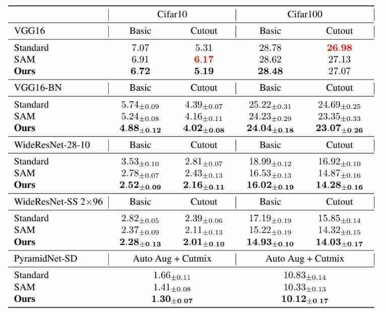
The author of the paper is also in the current very popular network structure V i s i o n T r a n s f o r m e r \mathrm{Vision \text{ } Transformer} Vision Transformer Experiments were carried out . The following table shows in C i f a r 10 \mathrm{Cifar10} Cifar10 and C i f a r 100 \mathrm{Cifar100} Cifar100 These two datasets are different V i T \mathrm{ViT} ViT Network structure in standard training , S A M \mathrm{SAM} SAM Comparison of test error rate between the three training methods with gradient constraint in this paper . Similarly, it can also be found that the test error rate of the method proposed in this paper is the lowest in all cases , This shows that the method in this paper can also be mentioned V i s i o n t r a n s f o r m e r \mathrm{Vision \text{ } transformer} Vision transformer Generalization of model .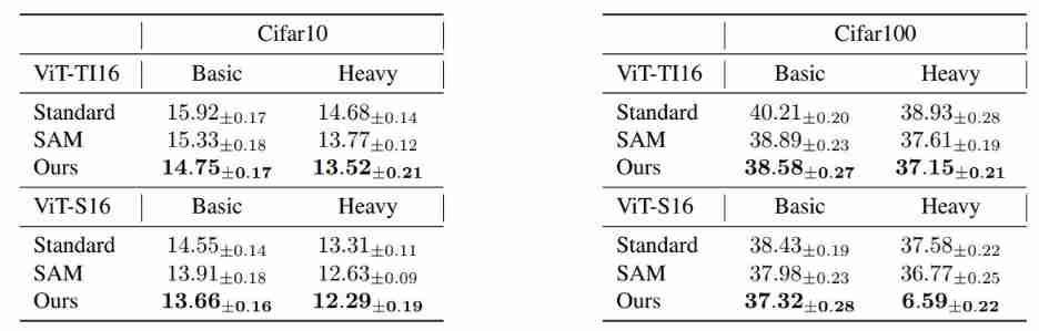
边栏推荐
- Sword finger offer 20 String representing numeric value
- Design and implementation of redis 7.0 multi part AOF
- There is no need to authorize the automatic dream weaving collection plug-in for dream weaving collection
- Yyds dry goods inventory override and virtual of classes in C
- Www 2022 | taxoenrich: self supervised taxonomy complemented by Structural Semantics
- Enhanced for loop
- 求esp32C3板子連接mssql方法
- Chapter 3.4: starrocks data import - Flink connector and CDC second level data synchronization
- 機器學習基礎:用 Lasso 做特征選擇
- Final consistency of MESI cache in CPU -- why does CPU need cache
猜你喜欢

On Valentine's day, I code a programmer's exclusive Bing Dwen Dwen (including the source code for free)

Ai aide à la recherche de plagiat dans le design artistique! L'équipe du professeur Liu Fang a été embauchée par ACM mm, une conférence multimédia de haut niveau.

Talking about custom conditions and handling errors in MySQL Foundation

MySQL advanced SQL statement (1)

WordPress collection WordPress hang up collection plug-in
Write the first CUDA program
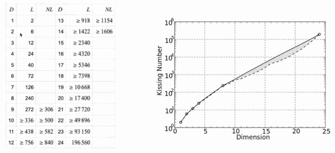
Kiss number + close contact problem
C language black Technology: Archimedes spiral! Novel, interesting, advanced~

7 * 24-hour business without interruption! Practice of applying multiple live landing in rookie villages
![[Yugong series] February 2022 attack and defense world advanced question misc-83 (QR easy)](/img/36/e5b716f2f976eb474b673f85363dae.jpg)
[Yugong series] February 2022 attack and defense world advanced question misc-83 (QR easy)
随机推荐
[untitled]
13. Time conversion function
PTA tiantisai l1-079 tiantisai's kindness (20 points) detailed explanation
Intel's new GPU patent shows that its graphics card products will use MCM Packaging Technology
查詢效率提昇10倍!3種優化方案,幫你解决MySQL深分頁問題
Imperial cms7.5 imitation "D9 download station" software application download website source code
在尋求人類智能AI的過程中,Meta將賭注押向了自監督學習
Learn these super practical Google browser skills, girls casually flirt
Kiss number + close contact problem
The reasons why QT fails to connect to the database and common solutions
Chapter 3.4: starrocks data import - Flink connector and CDC second level data synchronization
LV1 tire pressure monitoring
Write the first CUDA program
Base d'apprentissage de la machine: sélection de fonctionnalités avec lasso
Gee import SHP data - crop image
Final consistency of MESI cache in CPU -- why does CPU need cache
150 ppt! The most complete "fair perception machine learning and data mining" tutorial, Dr. AIST Toshihiro kamishima, Japan
Johnson–Lindenstrauss Lemma
Take you to master the formatter of visual studio code
C learning notes: C foundation - Language & characteristics interpretation