当前位置:网站首页>《MATLAB 神經網絡43個案例分析》:第42章 並行運算與神經網絡——基於CPU/GPU的並行神經網絡運算
《MATLAB 神經網絡43個案例分析》:第42章 並行運算與神經網絡——基於CPU/GPU的並行神經網絡運算
2022-07-02 03:23:00 【mozun2020】
《MATLAB 神經網絡43個案例分析》:第42章 並行運算與神經網絡——基於CPU/GPU的並行神經網絡運算
1. 前言
《MATLAB 神經網絡43個案例分析》是MATLAB技術論壇(www.matlabsky.com)策劃,由王小川老師主導,2013年北京航空航天大學出版社出版的關於MATLAB為工具的一本MATLAB實例教學書籍,是在《MATLAB神經網絡30個案例分析》的基礎上修改、補充而成的,秉承著“理論講解—案例分析—應用擴展”這一特色,幫助讀者更加直觀、生動地學習神經網絡。
《MATLAB神經網絡43個案例分析》共有43章,內容涵蓋常見的神經網絡(BP、RBF、SOM、Hopfield、Elman、LVQ、Kohonen、GRNN、NARX等)以及相關智能算法(SVM、决策樹、隨機森林、極限學習機等)。同時,部分章節也涉及了常見的優化算法(遺傳算法、蟻群算法等)與神經網絡的結合問題。此外,《MATLAB神經網絡43個案例分析》還介紹了MATLAB R2012b中神經網絡工具箱的新增功能與特性,如神經網絡並行計算、定制神經網絡、神經網絡高效編程等。
近年來隨著人工智能研究的興起,神經網絡這個相關方向也迎來了又一陣研究熱潮,由於其在信號處理領域中的不俗錶現,神經網絡方法也在不斷深入應用到語音和圖像方向的各種應用當中,本文結合書中案例,對其進行仿真實現,也算是進行一次重新學習,希望可以溫故知新,加强並提昇自己對神經網絡這一方法在各領域中應用的理解與實踐。自己正好在多抓魚上入手了這本書,下面開始進行仿真示例,主要以介紹各章節中源碼應用示例為主,本文主要基於MATLAB2018a(64比特,MATLAB2015b未安裝並行處理工具箱)平臺仿真實現,這是本書第四十二章並行運算與神經網絡實例,話不多說,開始!
2. MATLAB 仿真示例一
打開MATLAB,點擊“主頁”,點擊“打開”,找到示例文件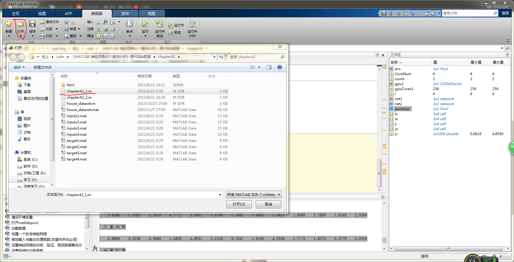
選中chapter42_1.m,點擊“打開”
chapter42_1.m源碼如下:
%%%%%%%%%%%%%%%%%%%%%%%%%%%%%%%%%%%%%%%%%%%%%%%%%%%%
%功能:並行運算與神經網絡-基於CPU/GPU的並行神經網絡運算
%環境:Win7,Matlab2015b
%Modi: C.S
%時間:2022-06-21
%%%%%%%%%%%%%%%%%%%%%%%%%%%%%%%%%%%%%%%%%%%%%%%%%%%%


%% Matlab神經網絡43個案例分析

% 並行運算與神經網絡-基於CPU/GPU的並行神經網絡運算
% by 王小川(@王小川_matlab)
% http://www.matlabsky.com
% Email:[email protected]163.com
% http://weibo.com/hgsz2003
% 本代碼為示例代碼脚本,建議不要整體運行,運行時注意備注提示。
close all;
clear all
clc

tic
%% CPU並行
%% 標准單線程的神經網絡訓練與仿真過程
[x,t]=house_dataset;
net1=feedforwardnet(10);
net2=train(net1,x,t);
y=sim(net2,x);

%% 打開MATLAB workers
% matlabpool open

% 檢查worker數量
delete(gcp('nocreate'))
poolsize=parpool(2)

%% 設置train與sim函數中的參數“Useparallel”為“yes”。
net2=train(net1,x,t,'Useparallel','yes')
y=sim(net2,x,'Useparallel','yes');

%% 使用“showResources”選項證實神經網絡運算確實在各個worker上運行。
net2=train(net1,x,t,'useParallel','yes','showResources','yes');
y=sim(net2,x,'useParallel','yes','showResources','yes');

%% 將一個數據集進行隨機劃分,同時保存到不同的文件
CoreNum=2; %設定機器CPU核心數量
if isempty(gcp('nocreate'))
    parpool(CoreNum);
end
for i=1:2
x=rand(2,1000);
save(['inputs' num2str(i)],'x')
t=x(1,:).*x(2,:)+2*(x(1,:)+x(2,:)) ;
save(['target' num2str(i)],'t');
clear x t
end

%% 實現並行運算加載數據集
CoreNum=2; %設定機器CPU核心數量
if isempty(gcp('nocreate'))
    parpool(CoreNum);
end
for i=1:2
    data=load(['inputs' num2str(i)],'x');
    xc{
    i}=data.x;
    data=load(['target' num2str(i)],'t');
    tc{
    i}=data.t;
    clear data
end
net2=configure(net2,xc{
    1},tc{
    1});
net2=train(net2,xc,tc);
yc=sim(net2,xc);

%% 得到各個worker返回的Composite結果
CoreNum=2; %設定機器CPU核心數量
if isempty(gcp('nocreate'))
    parpool(CoreNum);
end
for i=1:2
    yi=yc{
    i};
end

%% GPU並行
count=gpuDeviceCount
gpu1=gpuDevice(1)
gpuCores1=gpu1.MultiprocessorCount*gpu1.SIMDWidth
net2=train(net1,xc,tc,'useGPU','yes')
y=sim(net2,xc,'useGPU','yes')
net1.trainFcn='trainscg';
net2=train(net1,xc,tc,'useGPU','yes','showResources','yes');
y=sim(net2,xc, 'useGPU','yes','showResources','yes');
toc
添加完畢,點擊“運行”,開始仿真,輸出仿真結果如下:
Parallel pool using the 'local' profile is shutting down.
Starting parallel pool (parpool) using the 'local' profile ...
connected to 2 workers.

poolsize =

 Pool - 屬性:

            Connected: true
           NumWorkers: 2
              Cluster: local
        AttachedFiles: {
    }
    AutoAddClientPath: true
          IdleTimeout: 30 minutes (30 minutes remaining)
          SpmdEnabled: true


net2 =

    Neural Network

              name: 'Feed-Forward Neural Network'
          userdata: (your custom info)

    dimensions:

         numInputs: 1
         numLayers: 2
        numOutputs: 1
    numInputDelays: 0
    numLayerDelays: 0
 numFeedbackDelays: 0
 numWeightElements: 151
        sampleTime: 1

    connections:

       biasConnect: [1; 1]
      inputConnect: [1; 0]
      layerConnect: [0 0; 1 0]
     outputConnect: [0 1]

    subobjects:

             input: Equivalent to inputs{
    1}
            output: Equivalent to outputs{
    2}

            inputs: {
    1x1 cell array of 1 input}
            layers: {
    2x1 cell array of 2 layers}
           outputs: {
    1x2 cell array of 1 output}
            biases: {
    2x1 cell array of 2 biases}
      inputWeights: {
    2x1 cell array of 1 weight}
      layerWeights: {
    2x2 cell array of 1 weight}

    functions:

          adaptFcn: 'adaptwb'
        adaptParam: (none)
          derivFcn: 'defaultderiv'
         divideFcn: 'dividerand'
       divideParam: .trainRatio, .valRatio, .testRatio
        divideMode: 'sample'
           initFcn: 'initlay'
        performFcn: 'mse'
      performParam: .regularization, .normalization
          plotFcns: {
    'plotperform', plottrainstate, ploterrhist,
                    plotregression}
        plotParams: {
    1x4 cell array of 4 params}
          trainFcn: 'trainlm'
        trainParam: .showWindow, .showCommandLine, .show, .epochs,
                    .time, .goal, .min_grad, .max_fail, .mu, .mu_dec,
                    .mu_inc, .mu_max

    weight and bias values:

                IW: {
    2x1 cell} containing 1 input weight matrix
                LW: {
    2x2 cell} containing 1 layer weight matrix
                 b: {
    2x1 cell} containing 2 bias vectors

    methods:

             adapt: Learn while in continuous use
         configure: Configure inputs & outputs
            gensim: Generate Simulink model
              init: Initialize weights & biases
           perform: Calculate performance
               sim: Evaluate network outputs given inputs
             train: Train network with examples
              view: View diagram
       unconfigure: Unconfigure inputs & outputs


Computing Resources:
Parallel Workers:
  Worker 1 on 123-PC, MEX on PCWIN64
  Worker 2 on 123-PC, MEX on PCWIN64


Computing Resources:
Parallel Workers:
  Worker 1 on 123-PC, MEX on PCWIN64
  Worker 2 on 123-PC, MEX on PCWIN64


count =

     2


gpu1 =

  CUDADevice - 屬性:

                      Name: 'GeForce GTX 960'
                     Index: 1
         ComputeCapability: '5.2'
            SupportsDouble: 1
             DriverVersion: 10.2000
            ToolkitVersion: 9
        MaxThreadsPerBlock: 1024
          MaxShmemPerBlock: 49152
        MaxThreadBlockSize: [1024 1024 64]
               MaxGridSize: [2.1475e+09 65535 65535]
                 SIMDWidth: 32
               TotalMemory: 4.2950e+09
           AvailableMemory: 3.2666e+09
       MultiprocessorCount: 8
              ClockRateKHz: 1266000
               ComputeMode: 'Default'
      GPUOverlapsTransfers: 1
    KernelExecutionTimeout: 1
          CanMapHostMemory: 1
           DeviceSupported: 1
            DeviceSelected: 1


gpuCores1 =

   256

NOTICE: Jacobian training not supported on GPU. Training function set to TRAINSCG.

net2 =

    Neural Network

              name: 'Feed-Forward Neural Network'
          userdata: (your custom info)

    dimensions:

         numInputs: 1
         numLayers: 2
        numOutputs: 1
    numInputDelays: 0
    numLayerDelays: 0
 numFeedbackDelays: 0
 numWeightElements: 41
        sampleTime: 1

    connections:

       biasConnect: [1; 1]
      inputConnect: [1; 0]
      layerConnect: [0 0; 1 0]
     outputConnect: [0 1]

    subobjects:

             input: Equivalent to inputs{
    1}
            output: Equivalent to outputs{
    2}

            inputs: {
    1x1 cell array of 1 input}
            layers: {
    2x1 cell array of 2 layers}
           outputs: {
    1x2 cell array of 1 output}
            biases: {
    2x1 cell array of 2 biases}
      inputWeights: {
    2x1 cell array of 1 weight}
      layerWeights: {
    2x2 cell array of 1 weight}

    functions:

          adaptFcn: 'adaptwb'
        adaptParam: (none)
          derivFcn: 'defaultderiv'
         divideFcn: 'dividerand'
       divideParam: .trainRatio, .valRatio, .testRatio
        divideMode: 'sample'
           initFcn: 'initlay'
        performFcn: 'mse'
      performParam: .regularization, .normalization
          plotFcns: {
    'plotperform', plottrainstate, ploterrhist,
                    plotregression}
        plotParams: {
    1x4 cell array of 4 params}
          trainFcn: 'trainscg'
        trainParam: .showWindow, .showCommandLine, .show, .epochs,
                    .time, .goal, .min_grad, .max_fail, .sigma,
                    .lambda

    weight and bias values:

                IW: {
    2x1 cell} containing 1 input weight matrix
                LW: {
    2x2 cell} containing 1 layer weight matrix
                 b: {
    2x1 cell} containing 2 bias vectors

    methods:

             adapt: Learn while in continuous use
         configure: Configure inputs & outputs
            gensim: Generate Simulink model
              init: Initialize weights & biases
           perform: Calculate performance
               sim: Evaluate network outputs given inputs
             train: Train network with examples
              view: View diagram
       unconfigure: Unconfigure inputs & outputs


y =

  1×2 cell 數組

    {
    1×1000 double}    {
    1×1000 double}


Computing Resources:
GPU device #1, GeForce GTX 960


Computing Resources:
GPU device #1, GeForce GTX 960

時間已過 70.246120 秒。
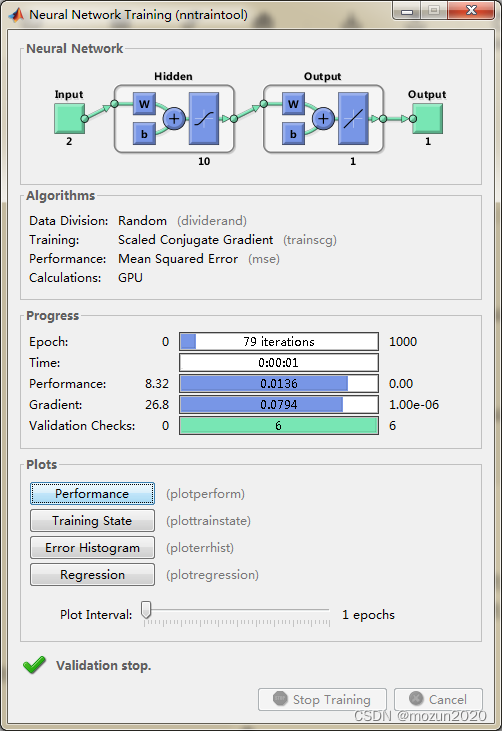
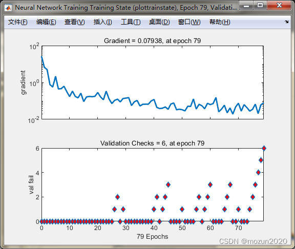
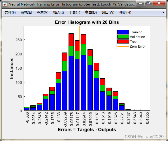
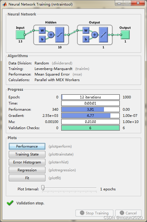
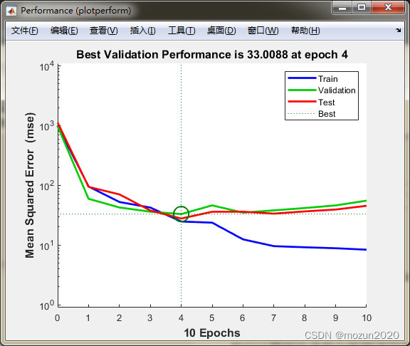
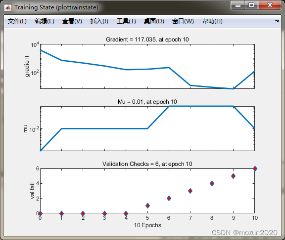
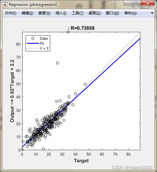
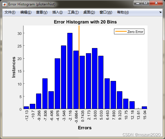
依次點擊Plots中的Performance,Training State,Error Histogram,Regression可得到如下圖示:

3. MATLAB 仿真示例二
選中並打開MATLAB當前文件夾視圖中chapter42_2.m,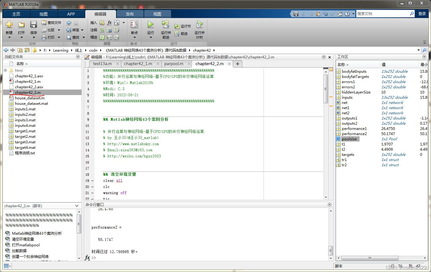
chapter42_2.m源碼如下:
%%%%%%%%%%%%%%%%%%%%%%%%%%%%%%%%%%%%%%%%%%%%%%%%%%%%
%功能:並行運算與神經網絡-基於CPU/GPU的並行神經網絡運算
%環境:Win7,Matlab2015b
%Modi: C.S
%時間:2022-06-21
%%%%%%%%%%%%%%%%%%%%%%%%%%%%%%%%%%%%%%%%%%%%%%%%%%%%
%% Matlab神經網絡43個案例分析
% 並行運算與神經網絡-基於CPU/GPU的並行神經網絡運算
% by 王小川(@王小川_matlab)
% http://www.matlabsky.com
% Email:[email protected]163.com
% http://weibo.com/hgsz2003
%% 清空環境變量
clear all
clc
warning off
tic
%% 打開matlabpool
% matlabpool open
delete(gcp('nocreate'))
poolsize=parpool(2)
%% 加載數據
load bodyfat_dataset
inputs = bodyfatInputs;
targets = bodyfatTargets;
%% 創建一個擬合神經網絡
hiddenLayerSize = 10; % 隱藏層神經元個數為10
net = fitnet(hiddenLayerSize); % 創建網絡
%% 指定輸入與輸出處理函數(本操作並非必須)
net.inputs{
1}.processFcns = {
'removeconstantrows','mapminmax'};
net.outputs{
2}.processFcns = {
'removeconstantrows','mapminmax'};
%% 設置神經網絡的訓練、驗證、測試數據集劃分
net.divideFcn = 'dividerand'; % 隨機劃分數據集
net.divideMode = 'sample'; % 劃分單比特為每一個數據
net.divideParam.trainRatio = 70/100; %訓練集比例
net.divideParam.valRatio = 15/100; %驗證集比例
net.divideParam.testRatio = 15/100; %測試集比例
%% 設置網絡的訓練函數
net.trainFcn = 'trainlm'; % Levenberg-Marquardt
%% 設置網絡的誤差函數
net.performFcn = 'mse'; % Mean squared error
%% 設置網絡可視化函數
net.plotFcns = {
'plotperform','plottrainstate','ploterrhist', ...
'plotregression', 'plotfit'};
%% 單線程網絡訓練
tic
[net1,tr1] = train(net,inputs,targets);
t1=toc;
disp(['單線程神經網絡的訓練時間為',num2str(t1),'秒']);
%% 並行網絡訓練
tic
[net2,tr2] = train(net,inputs,targets,'useParallel','yes','showResources','yes');
t2=toc;
disp(['並行神經網絡的訓練時間為',num2str(t2),'秒']);
%% 網絡效果驗證
outputs1 = sim(net1,inputs);
outputs2 = sim(net2,inputs);
errors1 = gsubtract(targets,outputs1);
errors2 = gsubtract(targets,outputs2);
performance1 = perform(net1,targets,outputs1);
performance2 = perform(net2,targets,outputs2);
%% 神經網絡可視化
figure, plotperform(tr1);
figure, plotperform(tr2);
figure, plottrainstate(tr1);
figure, plottrainstate(tr2);
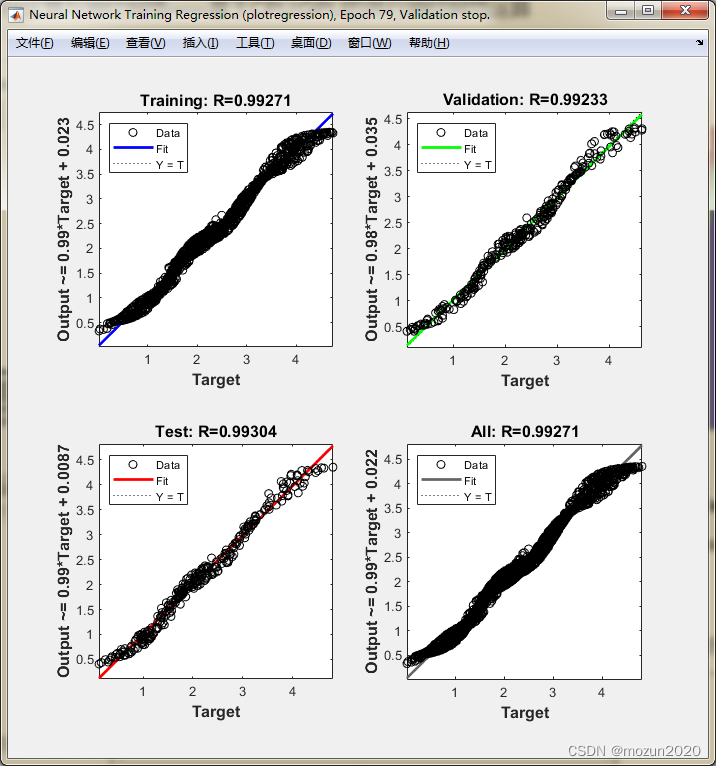
figure,plotregression(targets,outputs1);
figure,plotregression(targets,outputs2);
figure,ploterrhist(errors1);
figure,ploterrhist(errors2);
toc
% matlabpool close
點擊“運行”,開始仿真,輸出仿真結果如下:
Parallel pool using the 'local' profile is shutting down.
Starting parallel pool (parpool) using the 'local' profile ...
connected to 2 workers.

poolsize =

 Pool - 屬性:

            Connected: true
           NumWorkers: 2
              Cluster: local
        AttachedFiles: {
    }
    AutoAddClientPath: true
          IdleTimeout: 30 minutes (30 minutes remaining)
          SpmdEnabled: true

單線程神經網絡的訓練時間為1.9707秒

Computing Resources:
Parallel Workers:
  Worker 1 on 123-PC, MEX on PCWIN64
  Worker 2 on 123-PC, MEX on PCWIN64

並行神經網絡的訓練時間為4.4909秒

performance1 =

   26.4750


performance2 =

   50.1747

時間已過 12.766995 秒。


4. 小結
並行計算相關函數與數據調用在MATLAB2015版本之後都有昇級,所以需要對源碼進行調整再進行仿真,本文示例均根據機器情况與MATLAB版本進行適配。對本章內容感興趣或者想充分學習了解的,建議去研習書中第四十二章節的內容。後期會對其中一些知識點在自己理解的基礎上進行補充,歡迎大家一起學習交流。
边栏推荐
- C # joint halcon out of halcon Environment and various Error Reporting and Resolution Experiences
- venn图取交集
- On redis (II) -- cluster version
- Halcon image rectification
- Global and Chinese market of gynaecological health training manikin 2022-2028: Research Report on technology, participants, trends, market size and share
- Competition and adventure burr
- SAML2.0 notes (I)
- KL divergence is a valuable article
- Global and Chinese markets for hand hygiene monitoring systems 2022-2028: Research Report on technology, participants, trends, market size and share
- Calculation of page table size of level 2, level 3 and level 4 in protection mode (4k=4*2^10)
猜你喜欢
SAML2.0 笔记(一)

Verilog 状态机
Verilog 避免 Latch
![[JS reverse series] analysis of a customs publicity platform](/img/15/fdff7047e789d4e7c3c273a2f714f3.jpg)
[JS reverse series] analysis of a customs publicity platform
Verilog timing control
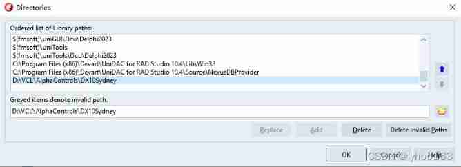
Delphi xe10.4 installing alphacontrols15.12

Discussion on related configuration of thread pool
verilog 并行块实现
高并发场景下缓存处理方案

Large screen visualization from bronze to the advanced king, you only need a "component reuse"!
随机推荐
旋转框目标检测mmrotate v0.3.1 学习模型
JDBC details
Verilog 过程连续赋值
Global and Chinese market of bone adhesives 2022-2028: Research Report on technology, participants, trends, market size and share
3124. Word list
Redis cluster
/silicosis/geo/GSE184854_ scRNA-seq_ mouse_ lung_ ccr2/GSE184854_ RAW/GSM5598265_ matrix_ inflection_ demult
Kotlin基础学习 14
aaaaaaaaaaaaa
焱融看 | 混合云时代下,如何制定多云策略
Redis set command line operation (intersection, union and difference, random reading, etc.)
Named block Verilog
PY3, PIP appears when installing the library, warning: ignoring invalid distribution -ip
焱融看 | 混合雲時代下,如何制定多雲策略
MySQL advanced (Advanced) SQL statement (II)
Verilog avoid latch
创业了...
Exchange rate query interface
Intersection of Venn graph
halcon图像矫正