当前位置:网站首页>Deep learning ----- using NN, CNN, RNN neural network to realize MNIST data set processing
Deep learning ----- using NN, CNN, RNN neural network to realize MNIST data set processing
2022-07-03 23:23:00 【Xiaofeilong programmer】
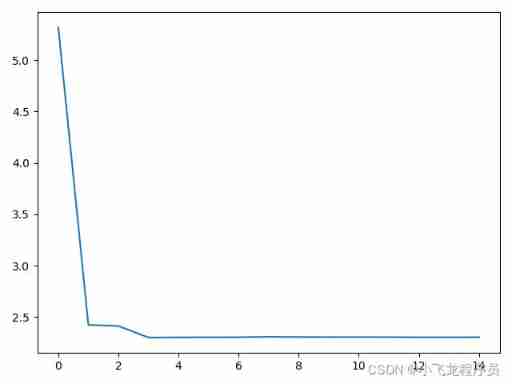
1. use NN The neural network completes MNIST Dataset processing
#  use NN The neural network completes MNIST Dataset processing
# 1、 Guide pack
import tensorflow as tf
import numpy as np
import matplotlib.pyplot as plt
from tensorflow.examples.tutorials.mnist import input_data
# 2、 load mnist Data sets
mnist=input_data.read_data_sets('mnist_data',one_hot=True)
x_data=mnist.train.images
y_data=mnist.train.labels
# 3、 Set up a place holder
x=tf.placeholder(tf.float32,shape=[None,28*28])
y=tf.placeholder(tf.float32,shape=[None,10])
# 4、 Set offset weights
w1=tf.Variable(tf.random_normal([28*28,200]))
b1=tf.Variable(tf.random_normal([200]))

w2=tf.Variable(tf.random_normal([200,100]))
b2=tf.Variable(tf.random_normal([100]))

w3=tf.Variable(tf.random_normal([100,10]))
b3=tf.Variable(tf.random_normal([10]))
# 5、 Set the prediction model
a1=tf.tanh(tf.matmul(x,w1)+b1)
a2=tf.tanh(tf.matmul(a1,w2)+b2)
a3=tf.matmul(a2,w3)+b3

# 6、 Cost function
cost=tf.reduce_mean(tf.nn.softmax_cross_entropy_with_logits(logits=a3,labels=y))

# 7、 Small batch gradient descent
# optimiter=tf.train.AdamOptimizer(learning_rate=0.001).minimize(cost)
dz3=a3-y
dw3=tf.matmul(tf.transpose(a2),dz3)/tf.cast(tf.shape(a2)[0],dtype=tf.float32)
db3=tf.reduce_mean(dz3,axis=0)

da2=tf.matmul(dz3,tf.transpose(w3))
dz2=da2*a2*(1-a2)
dw2=tf.matmul(tf.transpose(a1),dz2)/tf.cast(tf.shape(a1)[0],dtype=tf.float32)
db2=tf.reduce_mean(dz2,axis=0)

da1=tf.matmul(dz2,tf.transpose(w2))
dz1=da1*a1*(1-a1)
dw1=tf.matmul(tf.transpose(x),dz1)/tf.cast(tf.shape(x)[0],dtype=tf.float32)
db1=tf.reduce_mean(dz1,axis=0)
learning=0.01
optimiter=[
    tf.assign(w3,w3-learning*dw3),
    tf.assign(w2,w2-learning*dw2),
    tf.assign(w1,w1-learning*dw1),
    tf.assign(b3,b3-learning*db3),
    tf.assign(b2,b2-learning*db2),
    tf.assign(b1,b1-learning*db1),
]
# correct=tf.nn.in_top_k(a3,y,1)
# accuracy=tf.reduce_mean(tf.cast(correct,tf.float32))
y_true=tf.argmax(y,1)
y_predict=tf.argmax(a3,1)
accuracy=tf.reduce_mean(tf.cast(tf.equal(y_true,y_predict),tf.float32))
# 8、 Create a session
sess=tf.Session()
sess.run(tf.global_variables_initializer())
# 9、 Cycle output accuracy and cost
batch_size=100
train_count=20
ls=[]
for epo in range(train_count):
    avg_cost=0
    total_batch=mnist.train.num_examples//batch_size
    for i in range(total_batch):
        batch_x,batch_y=mnist.train.next_batch(batch_size)
        cost_val,_,acc=sess.run([cost,optimiter,accuracy],feed_dict={
    x:batch_x,y:batch_y})
        avg_cost+=cost_val/total_batch
    ls.append(avg_cost)
    print('epo:',epo,' On behalf of value :',avg_cost)
acc_v=sess.run(accuracy,feed_dict={
    x:mnist.test.images,y:mnist.test.labels})
print(acc_v)
# 10、 Draw the cost function diagram
plt.plot(ls)
plt.show()
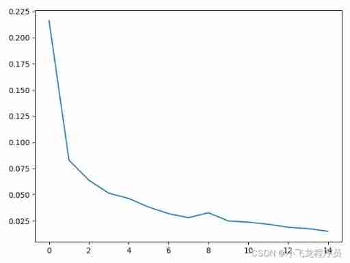
2. Complete with convolution neural network mnist Dataset processing
Method 1 :
# 1. Use convolution neural network to complete mnist Dataset processing
# 1、 Guide pack
import tensorflow as tf
import numpy as np
import matplotlib.pyplot as plt
from tensorflow.examples.tutorials.mnist import input_data
# 2、 Load data
mnist=input_data.read_data_sets('mnist_data',one_hot=True)
x_data=mnist.train.images
y_data=mnist.train.labels
# 3、 Set super parameters
width=28
height=28
# 4、 Define convolution placeholders
x=tf.placeholder(tf.float32,shape=[None,height*width])
y=tf.placeholder(tf.float32,shape=[None,10])
x_img=tf.reshape(x,[-1,width,height,1])
# 5、 Set the weight of the first layer , Convolution , Pooling layer
w1=tf.Variable(tf.random_normal([3,3,1,16]))
l1=tf.nn.conv2d(x_img,w1,strides=[1,1,1,1],padding='SAME')
l1=tf.nn.relu(l1)
l1=tf.nn.max_pool(l1,ksize=[1,2,2,1],strides=[1,2,2,1],padding='VALID')
# 6、 Set the second convolution , The weight , Pooling layer
w2=tf.Variable(tf.random_normal([3,3,16,32]))
l2=tf.nn.conv2d(l1,w2,strides=[1,1,1,1],padding='SAME')
l2=tf.nn.relu(l2)
l2=tf.nn.max_pool(l2,ksize=[1,2,2,1],strides=[1,2,2,1],padding='VALID')

dim=l2.get_shape()[1].value*l2.get_shape()[2].value*l2.get_shape()[3].value
l2_flat=tf.reshape(l2,[-1,dim])
# 7、 Set up the full connection layer
w3=tf.Variable(tf.random_normal([dim,100],stddev=0.01))
b3=tf.Variable(tf.random_normal([100]))
logit1=tf.matmul(l2_flat,w3)+b3

w4=tf.Variable(tf.random_normal([100,10],stddev=0.01))
b4=tf.Variable(tf.random_normal([10]))
logit2=tf.matmul(logit1,w4)+b4

# 8、 Set the cost function , Set the precision function
cost=tf.reduce_mean(tf.nn.softmax_cross_entropy_with_logits(logits=logit2,labels=y))
optimiter=tf.train.AdamOptimizer(learning_rate=0.001).minimize(cost)

y_true=tf.argmax(y,1)
y_predict=tf.argmax(logit2,1)
accuracy=tf.reduce_mean(tf.cast(tf.equal(y_true,y_predict),tf.float32))
# 9、 Small batch gradient descent training model
sess=tf.Session()
sess.run(tf.global_variables_initializer())
batch_size=100
train_count=15
ls=[]
for epo in range(train_count):
    avg_cost=0
    total_batch=mnist.train.num_examples//batch_size
    for i in range(total_batch):
        batch_x,batch_y=mnist.train.next_batch(batch_size)
        cost_val,_,acc=sess.run([cost,optimiter,accuracy],feed_dict={
    x:batch_x,y:batch_y})
        avg_cost+=cost_val/total_batch
    ls.append(avg_cost)
    print('epo:',epo,' On behalf of value :',avg_cost)

# 10、 Output accuracy and cost
acc_v=sess.run(accuracy,feed_dict={
    x:mnist.test.images,y:mnist.test.labels})
print(acc_v)
plt.plot(ls)
plt.show()
Method 2 :
# 1. Use convolution neural network to complete mnist Dataset processing (40 branch )
# 1、 Guide pack
import tensorflow as tf
import numpy as np
import matplotlib.pyplot as plt
from tensorflow.examples.tutorials.mnist import input_data
# 2、 Load data
mnist=input_data.read_data_sets('mnist_data')
x_data=mnist.train.images
y_data=mnist.train.labels
# 3、 Set super parameters
width=28
height=28
# 4、 Define convolution placeholders
x=tf.placeholder(tf.float32,shape=[None,height*width])
y=tf.placeholder(tf.int32,shape=[None])
x_img=tf.reshape(x,[-1,width,height,1])
# 5、 Set the weight of the first layer , Convolution , Pooling layer
w1=tf.Variable(tf.random_normal([3,3,1,16]))
l1=tf.nn.conv2d(x_img,w1,strides=[1,1,1,1],padding='SAME')
l1=tf.nn.relu(l1)
l1=tf.nn.max_pool(l1,ksize=[1,2,2,1],strides=[1,2,2,1],padding='VALID')
# 6、 Set the second convolution , The weight , Pooling layer
w2=tf.Variable(tf.random_normal([3,3,16,32]))
l2=tf.nn.conv2d(l1,w2,strides=[1,1,1,1],padding='SAME')
l2=tf.nn.relu(l2)
l2=tf.nn.max_pool(l2,ksize=[1,2,2,1],strides=[1,2,2,1],padding='VALID')

dim=l2.get_shape()[1].value*l2.get_shape()[2].value*l2.get_shape()[3].value
l2_flat=tf.reshape(l2,[-1,dim])
# 7、 Set up the full connection layer
w3=tf.Variable(tf.random_normal([dim,100],stddev=0.01))
b3=tf.Variable(tf.random_normal([100]))
logit1=tf.matmul(l2_flat,w3)+b3

w4=tf.Variable(tf.random_normal([100,10],stddev=0.01))
b4=tf.Variable(tf.random_normal([10]))
logit2=tf.matmul(logit1,w4)+b4

# 8、 Set the cost function , Set the precision function
cost=tf.reduce_mean(tf.nn.sparse_softmax_cross_entropy_with_logits(logits=logit2,labels=y))
optimiter=tf.train.AdamOptimizer(learning_rate=0.001).minimize(cost)

correct=tf.nn.in_top_k(logit2,y,1)# The prediction results of each sample are in the front of k Does the largest number contain targets Labels in forecasting
accuracy=tf.reduce_mean(tf.cast(correct,tf.float32))
# y_true=tf.argmax(y,1)
# y_predict=tf.argmax(logit2,1)
# accuracy=tf.reduce_mean(tf.cast(tf.equal(y_true,y_predict),tf.float32))
# 9、 Small batch gradient descent training model
sess=tf.Session()
sess.run(tf.global_variables_initializer())
batch_size=100
train_count=15
ls=[]
for epo in range(train_count):
    avg_cost=0
    total_batch=mnist.train.num_examples//batch_size
    for i in range(total_batch):
        batch_x,batch_y=mnist.train.next_batch(batch_size)
        cost_val,_,acc=sess.run([cost,optimiter,accuracy],feed_dict={
    x:batch_x,y:batch_y})
        avg_cost+=cost_val/total_batch
    ls.append(avg_cost)
    print('epo:',epo,' On behalf of value :',avg_cost)

# 10、 Output accuracy and cost
acc_v=sess.run(accuracy,feed_dict={
    x:mnist.test.images,y:mnist.test.labels})
print(acc_v)
plt.plot(ls)
plt.show()
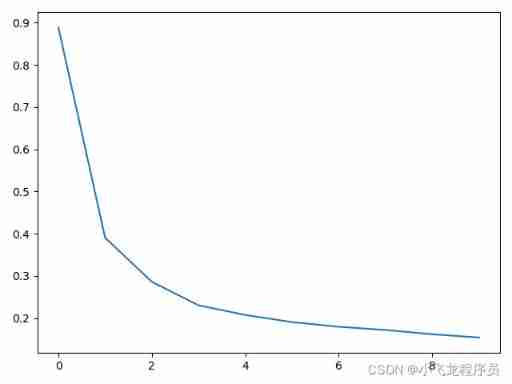
3. Complete with cyclic neural network mnist Dataset processing
Method 1 :
# 2. The processing cycle neural network is completed mnist Dataset processing (30 branch )
# 1、 Guide pack
import tensorflow as tf
from tensorflow.contrib.layers import fully_connected
from tensorflow.contrib.seq2seq import sequence_loss
from tensorflow.examples.tutorials.mnist import input_data
import matplotlib.pyplot as plt
# 2、 Load data
mnist=input_data.read_data_sets('mnist_data')
x_data=mnist.train.images
y_data=mnist.train.labels
# 3、 Set super parameters
n_input=28
steps=28
hidden_size=10
output_layer=10
# 4、 Place holder
x=tf.placeholder(tf.float32,shape=[None,steps,n_input])
y=tf.placeholder(tf.int32,shape=[None])
# 5、 Set up basic circulating nerve unit
# cell=tf.nn.rnn_cell.BasicRNNCell(num_units=hidden_size)
#cell=tf.nn.rnn_cell.BasicLSTMCell(num_units=hidden_size)
lstm_cell=[tf.nn.rnn_cell.LSTMCell(num_units=hidden_size) for layer in range(n_layers)]#10 Is the number of hidden layers
multi_cell=tf.nn.rnn_cell.MultiRNNCell(lstm_cell)
# 6、 Set up dynamic recurrent neural network
outputs,states=tf.nn.dynamic_rnn(multi_cell,x,dtype=tf.float32)
# 7、 Fully connected layer
logit=fully_connected(outputs[:,-1],output_layer,activation_fn=None)
# Cost function and optimizer
cost=tf.reduce_mean(tf.nn.sparse_softmax_cross_entropy_with_logits(logits=logit,labels=y))
optimiter=tf.train.AdamOptimizer(learning_rate=0.01).minimize(cost)
# 8、 Setting accuracy
correct=tf.nn.in_top_k(logit,y,1)
accuracy=tf.reduce_mean(tf.cast(correct,tf.float32))
# 9、 Small batch gradient descent training model
batch_size=100
train_count=10
ls=[]
with tf.Session() as sess:
    sess.run(tf.global_variables_initializer())
    for epo in range(train_count):
        avg_cost=0
        total_batch=mnist.train.num_examples//batch_size
        for i in range(total_batch):
            batch_x,batch_y=mnist.train.next_batch(batch_size)
            batch_x=batch_x.reshape([-1,28,28])
            cost_val,_,acc=sess.run([cost,optimiter,accuracy],feed_dict={
    x:batch_x,y:batch_y})
            avg_cost+=cost_val/total_batch
        ls.append(avg_cost)
        print('epo:',epo,' On behalf of value :',avg_cost,acc)
        acc_train=accuracy.eval(feed_dict={
    x:batch_x,y:batch_y})
        print('acc_train',acc_train)
        acc_test=sess.run(accuracy,feed_dict={
    x:mnist.test.images.reshape([-1,28,28]),y:mnist.test.labels})
        print('acc_test',acc_test)

# 10. Output accuracy , Cost function
plt.plot(ls)
plt.show()
Method 2 :
import tensorflow as tf
from tensorflow.contrib.layers import fully_connected
from tensorflow.contrib.seq2seq import sequence_loss
import numpy as np
from tensorflow.examples.tutorials.mnist import input_data
import random
#  stay tensorflow in , Using a recurrent neural network, multilayer LSTM How to achieve mnist Handwritten digit recognition .
# 1. Reading data (8 branch )
mnist=input_data.read_data_sets('mnist_data',one_hot=True)
x_data=mnist.train.images
y_data=mnist.train.labels
# 2. Define all parameters (8 branch )
n_inputs=28
n_steps=28
hidden_size=10
layers=4
n_outputs=10
# 3. Set up a place holder (8 branch )
x=tf.placeholder(tf.float32,shape=[None,n_steps,n_inputs])
y=tf.placeholder(tf.int32,shape=[None,None])
# 4. establish LSTMCell(8 branch )
cell=[tf.nn.rnn_cell.LSTMCell(num_units=hidden_size) for layer in range(layers)]
# 5. Stack multiple layers LSTMCell(8 branch )
multi_cell=tf.nn.rnn_cell.MultiRNNCell(cell)
outpus,states=tf.nn.dynamic_rnn(multi_cell,x,dtype=tf.float32)
# 6. Establish a full connection layer (8 branch )
logits=fully_connected(outpus[:,-1],n_outputs,activation_fn=None)
# 7. Calculate the cost or loss function (8 branch )
cost=tf.reduce_mean(tf.nn.softmax_cross_entropy_with_logits(logits=logits,labels=y))
optimiter=tf.train.AdamOptimizer(learning_rate=0.01).minimize(cost)
# 8. Set the accuracy model (8 branch )
y_true=tf.argmax(y,1)
y_predict=tf.argmax(logits,1)
accuracy=tf.reduce_mean(tf.cast(tf.equal(y_true,y_predict),tf.float32))
# correct=tf.nn.in_top_k(logits,y,1)
# accuracy=tf.reduce_mean(tf.cast(correct,tf.float32))
# 9. Use the training set data to train iterations 5 Time (8 branch )
train_count=5
batch_size=100
with tf.Session() as sess:
    sess.run(tf.global_variables_initializer())
    for epo in range(train_count):
        avg_cost=0
        total_batch=mnist.train.num_examples//batch_size
# 10. Training in batches , Each batch 100 Training samples (8 branch )
        for i in range(batch_size):
            batch_x,batch_y=mnist.train.next_batch(batch_size)
            batch_x=batch_x.reshape([-1,n_steps,n_inputs])
# 11. The accuracy of the output training set (6 branch )
            cost_val,_,acc=sess.run([cost,optimiter,accuracy],feed_dict={
    x:batch_x,y:batch_y})
            avg_cost+=cost_val/total_batch
        print(epo,avg_cost,acc)
    acc_train=accuracy.eval(feed_dict={
    x:batch_x,y:batch_y})
    print(acc_train)
# 12. The accuracy of the output test set (6 branch )
    acc_test = accuracy.eval(feed_dict={
    x: batch_x, y: batch_y})
    print(acc_test)
# 13. Take a sample from the test set for verification (8 branch )
    r=random.randint(0,mnist.test.num_examples-1)
    label = sess.run(tf.argmax(mnist.test.labels[r:r + 1], axis=2))
    predict=sess.run(tf.argmax(logits,2),feed_dict={
    x:mnist.test.images[r:r+1]})
    print(label,predict)

sess=tf.Session()
sess.run(tf.global_variables_initializer())
for epo in range(train_count):
    avg_cost=0
    total_batch=mnist.train.num_examples//batch_size
    for i in range(batch_size):
        batch_x,batch_y=mnist.train.next_batch(batch_size)
        batch_x=batch_x.reshape([-1,n_steps,n_inputs])
        cost_val,_=sess.run([cost,optimiter],feed_dict={
    x:batch_x,y:batch_y})
        avg_cost+=cost_val/total_batch
    acc_train = sess.run(accuracy,feed_dict={
    x: batch_x, y: batch_y})
    print(epo,avg_cost,'acc_train',acc_train)

acc_test=sess.run(accuracy,feed_dict={
    x:mnist.test.images.reshape([-1,n_steps,n_inputs]),y:mnist.test.labels})
print('acc_test',acc_test)
Be careful : Method 1 and method 2 are only modified in terms of parameters , The two methods have the same effect .
** The difference between the two methods :** Only the parameters have been adjusted
 Method 1 :
mnist=input_data.read_data_sets('mnist_data')
y=tf.placeholder(tf.int32,shape=[None,None])
cost=tf.reduce_mean(tf.nn.sparse_softmax_cross_entropy_with_logits(logits=logit,labels=y))
correct=tf.nn.in_top_k(logit,y,1)
accuracy=tf.reduce_mean(tf.cast(correct,tf.float32))
 Method 2 :
mnist=input_data.read_data_sets('mnist_data',one_hot=True)
y=tf.placeholder(tf.int32,shape=[None,None])
y_true=tf.argmax(y,1)
y_predict=tf.argmax(logits,1)
accuracy=tf.reduce_mean(tf.cast(tf.equal(y_true,y_predict),tf.float32))
4. summary
4.1 Two methods of small batch training :
 Method 1 :
train_count=5
batch_size=100
with tf.Session() as sess:
    sess.run(tf.global_variables_initializer())
    for epo in range(train_count):
        avg_cost=0
        total_batch=mnist.train.num_examples//batch_size
        for i in range(batch_size):
            batch_x,batch_y=mnist.train.next_batch(batch_size)
            batch_x=batch_x.reshape([-1,n_steps,n_inputs])
cost_val,_,acc=sess.run([cost,optimiter,accuracy],feed_dict={
    x:batch_x,y:batch_y})
            avg_cost+=cost_val/total_batch
        print(epo,avg_cost,acc)
    acc_train=accuracy.eval(feed_dict={
    x:batch_x,y:batch_y})
    print(acc_train)
    acc_test = accuracy.eval(feed_dict={
    x: batch_x, y: batch_y})
    print(acc_test)
 Method 2 :
sess=tf.Session()
sess.run(tf.global_variables_initializer())
for epo in range(train_count):
    avg_cost=0
    total_batch=mnist.train.num_examples//batch_size
    for i in range(batch_size):
        batch_x,batch_y=mnist.train.next_batch(batch_size)
        batch_x=batch_x.reshape([-1,n_steps,n_inputs])
        cost_val,_=sess.run([cost,optimiter],feed_dict={
    x:batch_x,y:batch_y})
        avg_cost+=cost_val/total_batch
    acc_train = sess.run(accuracy,feed_dict={
    x: batch_x, y: batch_y})
    print(epo,avg_cost,'acc_train',acc_train)

acc_test=sess.run(accuracy,feed_dict={
    x:mnist.test.images.reshape([-1,n_steps,n_inputs]),y:mnist.test.labels})
print('acc_test',acc_test)
4.2 Randomly select a sample from the test set for verification
 Randomly select a sample from the test set for verification
r=random.randint(0,mnist.test.num_examples-1)
label = sess.run(tf.argmax(mnist.test.labels[r:r + 1], axis=2))
predict=sess.run(tf.argmax(logits,2),feed_dict={
    x:mnist.test.images[r:r+1]})
print(label,predict)
边栏推荐
- Gorilla/mux framework (RK boot): add tracing Middleware
- How to switch between dual graphics cards of notebook computer
- Fashion cloud interview questions series - JS high-frequency handwritten code questions
- 炒股开户佣金优惠怎么才能获得,网上开户安全吗
- How to solve the problem of computer networking but showing no Internet connection
- Actual combat | use composite material 3 in application
- 2022.02.14
- Loop compensation - explanation and calculation of first-order, second-order and op amp compensation
- C # basic knowledge (2)
- . Net ADO splicing SQL statement with parameters
猜你喜欢

A preliminary study on the middleware of script Downloader

The reason why the computer runs slowly and how to solve it

Unique in China! Alibaba cloud container service enters the Forrester leader quadrant
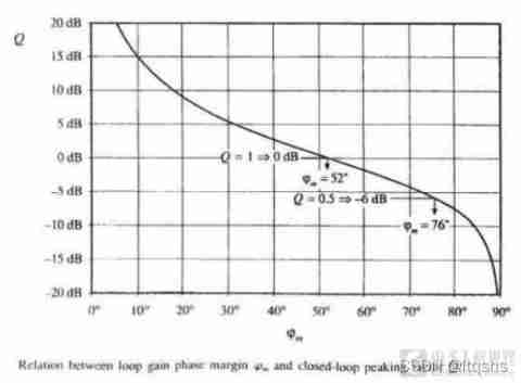
Loop compensation - explanation and calculation of first-order, second-order and op amp compensation
![[Android reverse] use DB browser to view and modify SQLite database (download DB browser installation package | install DB browser tool)](/img/1d/044e81258db86cf34eddd3b8f5cf90.jpg)
[Android reverse] use DB browser to view and modify SQLite database (download DB browser installation package | install DB browser tool)
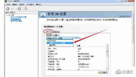
How to switch between dual graphics cards of notebook computer
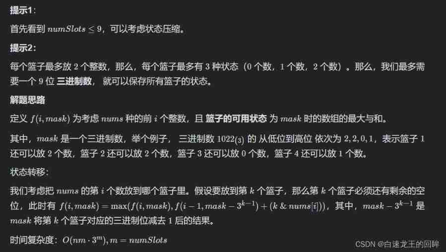
Leetcode week 4: maximum sum of arrays (shape pressing DP bit operation)

Firefox set up proxy server

How to quickly build high availability of service discovery

2022 chemical automation control instrument examination content and chemical automation control instrument simulation examination
随机推荐
Sword finger offer day 4 (Sword finger offer 03. duplicate numbers in the array, sword finger offer 53 - I. find the number I in the sorted array, and the missing numbers in sword finger offer 53 - ii
ADB command to get XML
Creation of the template of the password management software keepassdx
股票开户佣金最低的券商有哪些大家推荐一下,手机上开户安全吗
How to write a good title of 10w+?
Scratch uses runner Py run or debug crawler
How to quickly build high availability of service discovery
Subset enumeration method
"Learning notes" recursive & recursive
Weekly leetcode - nc9/nc56/nc89/nc126/nc69/nc120
Powerful blog summary
How to restore the factory settings of HP computer
D24:divisor and multiple (divisor and multiple, translation + solution)
2022 t elevator repair registration examination and the latest analysis of T elevator repair
Introduction to the gtid mode of MySQL master-slave replication
2022 free examination questions for hoisting machinery command and hoisting machinery command theory examination
Les sociétés de valeurs mobilières dont la Commission d'ouverture d'un compte d'actions est la plus faible ont ce que tout le monde recommande.
Programming language (2)
File copy method
How to quickly build high availability of service discovery