Implementation of support vector machine with ml11 sklearn

SKlearn library Realization SVM

%matplotlib inline 
# In order to be in notebook Chinese painting display 
import numpy as np
import matplotlib.pyplot as plt
from scipy import stats
import seaborn as sns; sns.set()

# Random data , Use sklearn Data points are randomly generated by the method under 
# among  cluster_std Is the degree of dispersion of data 
from sklearn.datasets.samples_generator import make_blobs
X, y = make_blobs(n_samples=50, centers=2,
                  random_state=0, cluster_std=0.60)
plt.scatter(X[:, 0], X[:, 1], c=y, s=50, cmap='autumn')

Train a basic SVM

# Classification task 
from sklearn.svm import SVC 
# Linear kernel function   Equivalent to not transforming the data 
model = SVC(kernel='linear')
model.fit(X, y)

Template of drawing function

# Plot function 
def plot_svc_decision_function(model, ax=None, plot_support=True):
   
    if ax is None:
        ax = plt.gca()
    xlim = ax.get_xlim()
    ylim = ax.get_ylim()
    
    #  use SVM Self contained decision_function Function to draw 
    x = np.linspace(xlim[0], xlim[1], 30)
    y = np.linspace(ylim[0], ylim[1], 30)
    Y, X = np.meshgrid(y, x)
    xy = np.vstack([X.ravel(), Y.ravel()]).T
    P = model.decision_function(xy).reshape(X.shape)
    
    #  Drawing decision boundaries 
    ax.contour(X, Y, P, colors='k',
               levels=[-1, 0, 1], alpha=0.5,
               linestyles=['--', '-', '--'])
    
    #  Drawing support vectors 
    if plot_support:
        ax.scatter(model.support_vectors_[:, 0],
                   model.support_vectors_[:, 1],
                   s=300, linewidth=1, alpha=0.2);
    ax.set_xlim(xlim)
    ax.set_ylim(ylim)

plt.scatter(X[:, 0], X[:, 1], c=y, s=50, cmap='autumn')
plot_svc_decision_function(model)

This line is the decision boundary we hope to get

It was observed that there was 3 Points are marked with special marks , They happen to be points on the boundary

They are ours support vectors（ Support vector ）

stay Scikit-Learn in , They are stored in this location support_vectors_（ An attribute ）

Observation can reveal , We only need support vectors to build the model

Next, let's try , Use different data points , See if the effect will change

Separate use 60 And 120 Data points

def plot_svm(N=10, ax=None):
    X, y = make_blobs(n_samples=200, centers=2,
                      random_state=0, cluster_std=0.60)
    X = X[:N]
    y = y[:N]
    model = SVC(kernel='linear', C=1E10)
    model.fit(X, y)
    
    ax = ax or plt.gca()
    ax.scatter(X[:, 0], X[:, 1], c=y, s=50, cmap='autumn')
    ax.set_xlim(-1, 4)
    ax.set_ylim(-1, 6)
    plot_svc_decision_function(model, ax)
#  Draw different data points respectively 
fig, ax = plt.subplots(1, 2, figsize=(16, 6))
fig.subplots_adjust(left=0.0625, right=0.95, wspace=0.1)
for axi, N in zip(ax, [60, 120]):
    plot_svm(N, axi)
    axi.set_title('N = {0}'.format(N))

Introducing kernel functions SVM

Plot another dataset distribution

from sklearn.datasets.samples_generator import make_circles
#  Draw another data set 
X, y = make_circles(100, factor=.1, noise=.1)
# Let's see if the linear sum function can solve this problem 
clf = SVC(kernel='linear').fit(X, y)

plt.scatter(X[:, 0], X[:, 1], c=y, s=50, cmap='autumn')
plot_svc_decision_function(clf, plot_support=False);

# Added a new dimension r
from mpl_toolkits import mplot3d
r = np.exp(-(X ** 2).sum(1))
#  Imagine stretching a circular dataset up and down in three dimensions 
def plot_3D(elev=30, azim=30, X=X, y=y):
    ax = plt.subplot(projection='3d')
    ax.scatter3D(X[:, 0], X[:, 1], r, c=y, s=50, cmap='autumn')
    ax.view_init(elev=elev, azim=azim)
    ax.set_xlabel('x')
    ax.set_ylabel('y')
    ax.set_zlabel('r')

plot_3D(elev=45, azim=45, X=X, y=y)

# Add Gaussian kernel 
clf = SVC(kernel='rbf')
clf.fit(X, y)

# This time it's great ！
plt.scatter(X[:, 0], X[:, 1], c=y, s=50, cmap='autumn')
plot_svc_decision_function(clf)
plt.scatter(clf.support_vectors_[:, 0], clf.support_vectors_[:, 1],
            s=300, lw=1, facecolors='none');

Adjust the SVM Parameters

#  This data set cluster_std A little bigger , In this way, the function of soft interval can be reflected 
X, y = make_blobs(n_samples=100, centers=2,
                  random_state=0, cluster_std=0.8)
plt.scatter(X[:, 0], X[:, 1], c=y, s=50, cmap='autumn')

C Parameters

# Data sets that make the game more difficult 
X, y = make_blobs(n_samples=100, centers=2,
                  random_state=0, cluster_std=0.8)

fig, ax = plt.subplots(1, 2, figsize=(16, 6))
fig.subplots_adjust(left=0.0625, right=0.95, wspace=0.1)
#  Select two C Parameters to carry out the opposite experiment , Respectively 10 and 0.1
for axi, C in zip(ax, [10.0, 0.1]):
    model = SVC(kernel='linear', C=C).fit(X, y)
    axi.scatter(X[:, 0], X[:, 1], c=y, s=50, cmap='autumn')
    plot_svc_decision_function(model, axi)
    axi.scatter(model.support_vectors_[:, 0],
                model.support_vectors_[:, 1],
                s=300, lw=1, facecolors='none');
    axi.set_title('C = {0:.1f}'.format(C), size=14)

Karma parameter , The larger the mapping, the higher the dimension , The more complex the model .

X, y = make_blobs(n_samples=100, centers=2,
                  random_state=0, cluster_std=1.1)

fig, ax = plt.subplots(1, 2, figsize=(16, 6))
fig.subplots_adjust(left=0.0625, right=0.95, wspace=0.1)
#  Choose different gamma Value to observe the modeling effect 
for axi, gamma in zip(ax, [10.0, 0.1]):
    model = SVC(kernel='rbf', gamma=gamma).fit(X, y)
    axi.scatter(X[:, 0], X[:, 1], c=y, s=50, cmap='autumn')
    plot_svc_decision_function(model, axi)
    axi.scatter(model.support_vectors_[:, 0],
                model.support_vectors_[:, 1],
                s=300, lw=1, facecolors='none');
    axi.set_title('gamma = {0:.1f}'.format(gamma), size=14)

For relatively large karma value , The boundary is clearly divided , But the generalization ability is relatively low ; Smaller karma value , Wrong data points , But the generalization ability is strong , More useful .

Face recognition examples

# Reading data sets 
from sklearn.datasets import fetch_lfw_people
# Everyone's face has at least 60 individual 
faces = fetch_lfw_people(min_faces_per_person=60)
# Look at the scale of the data 
print(faces.target_names)
print(faces.images.shape)

# 3 That's ok 5 Column layout 
fig, ax = plt.subplots(3, 5)
for i, axi in enumerate(ax.flat):
    axi.imshow(faces.images[i], cmap='bone')
    axi.set(xticks=[], yticks=[],
            xlabel=faces.target_names[faces.target[i]])

from sklearn.svm import SVC
from sklearn.decomposition import PCA
from sklearn.pipeline import make_pipeline

# Dimensionality reduction 150 dimension 
pca = PCA(n_components=150, whiten=True, random_state=42)
svc = SVC(kernel='rbf', class_weight='balanced')
# First reduce the dimension and then SVM
model = make_pipeline(pca, svc)

Divide the data set

from sklearn.model_selection import train_test_split
Xtrain, Xtest, ytrain, ytest = train_test_split(faces.data, faces.target,
                                                random_state=40)

Use grid search cross-validation To choose our parameters , Traverse C Hegama , See which works well .

from sklearn.model_selection import GridSearchCV
param_grid = {
    'svc__C': [1, 5, 10],
              'svc__gamma': [0.0001, 0.0005, 0.001]}
grid = GridSearchCV(model, param_grid)

%time grid.fit(Xtrain, ytrain)
print(grid.best_params_)

After selection, use our model to make predictions .

model = grid.best_estimator_
yfit = model.predict(Xtest)
yfit.shape

Result display

fig, ax = plt.subplots(4, 6)
for i, axi in enumerate(ax.flat):
    axi.imshow(Xtest[i].reshape(62, 47), cmap='bone')
    axi.set(xticks=[], yticks=[])
    axi.set_ylabel(faces.target_names[yfit[i]].split()[-1],
                   color='black' if yfit[i] == ytest[i] else 'red')
fig.suptitle('Predicted Names; Incorrect Labels in Red', size=14);

from sklearn.metrics import classification_report
print(classification_report(ytest, yfit,
                            target_names=faces.target_names))

Precision value and recall rate

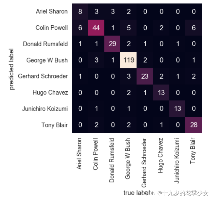
Confusion matrix

from sklearn.metrics import confusion_matrix
mat = confusion_matrix(ytest, yfit)
sns.heatmap(mat.T, square=True, annot=True, fmt='d', cbar=False,
            xticklabels=faces.target_names,
            yticklabels=faces.target_names)
plt.xlabel('true label')
plt.ylabel('predicted label');