Wuenda machine learning course - week 7

1. Support vector machine SVM

1.1 Optimization objectives

In logical regression , The loss function for a sample is as follows ：

​ $-y^{(i)}log(h_{\theta }(x^{(i)})+(1-y^{(i)})log(1-h_{\theta }(x^{(i)})=-y^{(i)}log(\frac{1}{1+e^{-{\theta }^T\cdot x}})+(1-y^{(i)})log(1-\frac{1}{1+e^{-{\theta }^T\cdot x}})$

Suppose $z={\theta }^T\cdot x$ Abscissa , The value of the above loss function is the ordinate , When $y$ Different images can be drawn with different values ：

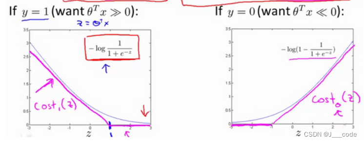
The blue curve in the above figure is the original image , The purplish red line is similar to the curve . If the new cost function is used to express the purple red line , It can be expressed as ： $\underset{\theta }{\min }C{\sum }_{i=1}^m\left[y^{(i)}{\mathrm{cost}}_1\left({\theta }^T{x}^{(i)}\right)+\left(1-y^{(i)}\right){\mathrm{cost}}_0\left({\theta }^T{x}^{(i)}\right)\right]+\frac{1}{2}{\sum }_{i=1}^n{\theta }_j^2$

​ The converted cost function is the cost function of support vector machine . among $cos{t}_1({\theta }^T{x}^{(i)})=-log{h}_{\theta }(x^{(i)}),cos{t}_0({\theta }^T{x}^{(i)})=-log(1-h_{\theta }(x^{(i)}))$, Respectively represent the purple red lines in the two subgraphs , And in the above formula, the constants in the front and back parts $\frac{1}{m}$ And in the regularization term $\lambda$ Delete , Change to... In Item 1 $C$, This is a SVM Common expressions , The actual meaning has not changed ： The original formula can be understood as $A+\lambda B$, If $\lambda$ A higher value indicates that $B$ The weight of the cost function is large ; Now change to $CA+B$, When $C$ The value of is small , Disguised increase $B$ The weight in the cost function , When $C=\frac{1}{\lambda }$ when , The two formulas will reach the same value when the gradient is updated

1.2 The intuitive understanding of the big boundary

The picture below is SVM The image of the cost function . When $y=1$ when ( Corresponding to left subgraph ), In order to minimize the loss value $z={\theta }^{T}x\ge 1$; When $y=0$ when ( Corresponding to right subgraph ), In order to minimize the loss value $z={\theta }^{T}x\le -1$. But in logistic regression, when $y=1$ when , Only required ${\theta }^{T}x\ge 0$ The sample can be correctly classified as a positive sample ; When $y=0$ when , Only required ${\theta }^{T}x<0$ The sample can be correctly classified as a negative sample ：

From the above analysis, we can see that SVM It's more demanding , Need one Safe spacing

When put $C$ When the value is set to a large value , At this point, it is necessary to find out that the first item is 0 Parameters of $\theta$. Suppose that the first item is chosen to be 0 Parameters of $\theta$, The constraints must be followed , When $y=1$ when ,${\theta }^{T}x\ge 1$ And when $y=0$ when ,${\theta }^{T}x\le -1$：

Why? SVM It is called a large spacing classifier ? For the dataset in the figure below , You can use multiple lines to separate positive and negative samples , See the purple red and green straight lines in the picture . Compared with these two lines, the black line visually separates the two types of samples better , Because there is a greater shortest distance between the black line and the sample ( There are two distance values from two types of samples , The smaller of these values ), signify SVM Robust , This distance is called SVM The distance between ：

When will $C$ When it is set very large , Outliers can seriously affect decision boundaries . In the following illustration , When $C$ large , The black line is the Red Cross not added to the lower left corner ( Outliers ) The resulting decision boundary . After adding outliers , In order to separate the samples with maximum spacing , The decision boundary changes from a black line to a purplish red line , It's obviously not very good ( It can be understood as over fitting ). So when $C$ When the set value is not very large , The influence of outliers can be ignored , Get a better decision boundary like the black line ：

1.3 The mathematics behind big boundary classification

First review the intuitive understanding of vector inner product , For two vectors $u=[u_1,u_2{]}^T,v=[v1,v2{]}^T$,$p$ by $v$ stay $u$ The projection on the ($p$ There are also positive and negative values , But not a vector ), be $u^{T}v=p\cdot ||u||=u_1{v}_1+u_2{v}_2$：

Now let's understand through the inner product property SVM The objective function of ：

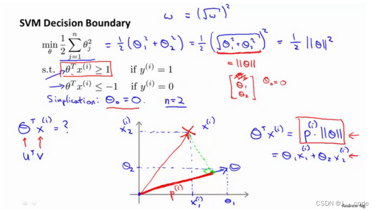
Let's start with ${\theta }_0=0$, And set the characteristic number to $n=2$, So the objective function is converted to :

​ $\underset{\theta }{\min }\frac{1}{2}{\sum }_{j=1}^n{\theta }_j^2=\frac{1}{2}({\theta }_1^2+{\theta }_2^2)=\frac{1}{2}({\sqrt{{\theta }_1^2+{\theta }_2^2)}}^2=\frac{1}{2}||\theta |{|}^2$

Through the previous intuitive introduction to inner product , constraint condition ${\theta }^T{x}^{(i)}=p^{(i)}||\theta ||$,$p^{(i)}$ Express $x^{(i)}$ stay $\theta$ The projection on the . So the objective function is as follows ：

Two types of samples in the left subgraph below , Suppose the green line is taken as the decision boundary ( namely ${\theta }^{T}x=0$, The reason why the green line goes through the origin here is because ${\theta }_0=0$), Then the blue vector $\theta$ Orthogonal to the green line , So a decision boundary corresponds to a parameter $\theta$ vector . Suppose the Red Cross is a positive sample , The blue circle is a negative sample , Then the positive sample in the figure $x^{(1)}$ And negative samples $x^{(2)}$ stay $\theta$ The length of the projection on is very short , To meet the $p^{(i)}||\theta ||\ge 1$ and $p^{(i)}||\theta ||\le -1$ You need to $||\theta ||$ The value of is very large , But the objective function is to $||\theta ||$ The value of is as small as possible , therefore $\theta$ The direction is not good ( That is, the choice of decision boundary is not good ).

SVM The decision boundary in the right subgraph below will be selected according to the objective function , Because the boundary makes $||\theta ||$ To become smaller ：

1.4 Kernel function Ⅰ

In order to obtain the decision boundary in the figure below , The model could be $h(\theta )={\theta }_0+{\theta }_1{x}_1+{\theta }_2{x}_2+{\theta }_3{x}_1{x}_2+...$ In the form of , Now suppose $f_1=x_1,f_2=x_2,f_3=x_1{x}_2,...$, be $h(\theta )={\theta }_0+{\theta }_1{f}_1+{\theta }_2{f}_2+...+{\theta }_n{f}_n$. In addition to combining the original features , Is there a better way to construct $f_1,f_2,...$？ This requires a kernel function

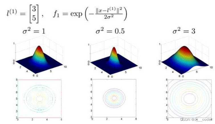
Suppose a sample is given $x$, utilize $x$ And pre selected tags $l^{(1)}、l^{(2)}、l^{(3)}$ The degree of approximation as $f_1、f_2、f_3$：

​ $f_1=\mathrm{similarity}\left(x,l^{(1)}\right)=e\left(-\frac{{\Vert x-l^{(1)}\Vert }^2}{2{\sigma }^2}\right)$

​ $f_2=\mathrm{similarity}\left(x,l^{(2)}\right)=e\left(-\frac{{\Vert x-l^{(2)}\Vert }^2}{2{\sigma }^2}\right)$

​ $f_3=\mathrm{similarity}\left(x,l^{(3)}\right)=e\left(-\frac{{\Vert x-l^{(3)}\Vert }^2}{2{\sigma }^2}\right)$

among ,$\mathrm{similarity}\left(x,l^{(i)}\right)$ It's a kernel function ( This function is a Gaussian kernel function ), Usually used $k(x,l^{(i)})$ Express . When $x$ Marking and marking $l^{(i)}$ The closer we get to , Characteristics $f_i$ Approximate to $e^{-0}=1$; When $x$ Marking and marking $l^{(i)}$ The farther away you are , Characteristics $f_i$ Approximate to $e^{-bignum}=0$. It can be understood intuitively from the following figure , When $l^{(1)}=[3,5{]}^T$ when , If $x=[3,5{]}^T$, be $z$ Axis Max ($z$ Axis representation $f_1$ Value ,$x$ and $y$ The axes are represented separately $x_1$ and $x_2$). in addition $\sigma$ The value of will control $f_1$ The value of the $x$ The rate of change ：

So how does the kernel function determine the decision boundary ？ Suppose that $h_{\theta }(x)={\theta }_0+{\theta }_1{f}_1+{\theta }_2{f}_2+{\theta }_3{f}_3$, At this point, the parameters are known , Respectively ${\theta }_0=0.5,{\theta }_1={\theta }_2=1,{\theta }_3=0$. For the purplish red sample points in the figure below , It can be seen that it is far from $l^{(1)}$ Closer , leave $l^{(2)}$ and $l^{(3)}$ Far away , therefore $f_1\approx 1,f_2\approx 0,f_3\approx 0$, therefore $h_{\theta }(x)>0$, That is, it is predicted that the sample point is a positive sample point . Similarly, green sample points are predicted as positive sample points , Blue and blue sample points are negative sample points , Finally, the red decision boundary . It can be seen that the characteristic value of the sample is not used in the above calculation $x_1、x_2、x_3$, Instead, new features calculated using kernel functions $f_1、f_2、f_3$：

1.5 Kernel function Ⅱ

stay 1.4 The concept and function of kernel function are introduced in this section , But I still don't know how to select tags $l^{(i)}$. The number of tags is usually selected according to the number of training sets , Suppose there is $m$ Samples , Then choose $m$ A sign , The new feature obtained in this way is based on the distance between a single sample point and all other sample points . Suppose each sample point is used as a marker , The new feature can be expressed as ：

therefore SVM The objective function of is converted to $\underset{\theta }{\min }C{\sum }_{i=1}^m\left[y^{(i)}{\mathrm{cost}}_1\left({\theta }^T{f}^{(i)}\right)+\left(1-y^{(i)}\right){\mathrm{cost}}_0\left({\theta }^T{f}^{(i)}\right)\right]+\frac{1}{2}{\sum }_{i=1}^{n=m}{\theta }_j^2$, And calculating ${\sum }_{i=1}^{n=m}{\theta }_j^2={\theta }^T\theta$ Will use ${\theta }^{T}M\theta$ To replace , Because of the simplified calculation , among $M$ Varies with the kernel function

​ Be careful ： When SVM When kernel functions are not used , It is called a linear kernel function , That is, the objective function or ${\theta }^{T}x$

Let's take a look $C=\frac{1}{\lambda }$ and $\sigma$ Yes SVM Influence ：

• When $C$ large , amount to $\lambda$ smaller , May cause over fitting , High variance
• When $C$ More hours , amount to $\lambda$ more , May lead to under fitting , High deviation
• When $\sigma$ large , features $f_i$ The change of is smooth , May lead to low variance , High deviation
• When $\sigma$ More hours , features $f_i$ The change of is more drastic , May cause low deviation , High variance

1.6 SVM Use

To use SVM, The following things must be done ：

• Choose the right one $C$ value
• Select kernel function ( It is also possible not to use kernel functions ), Kernel function except Gaussian kernel function , There are also polynomial kernel functions , But the goal is to build new features based on the distance between the sample and the marker
• Choose the right one $\sigma$ value

about SVM There are universal rules for the use of ,$m$ Sample size ,$n$ Characteristic number ：

• If $n$ Compare with $m$ It's much bigger , That is, the amount of data in the training set is not enough to support the training of a complex nonlinear model , The logistic regression model or the one without kernel function is used SVM

• If $n$ smaller ,$m$ Moderate size , Then the Gaussian kernel function is used SVM

• If $n$ smaller ,$m$ more , Then use SVM Will be very slow , More features need to be created , Then we use logistic regression or the function without kernel SVM

Neural network in the above three cases may have better performance , But training neural networks can be very slow , The main reason for choosing support vector machine is that its cost function is convex function , There is no local minimum

2. Reference resources

https://www.bilibili.com/video/BV164411b7dx?p=70-75

http://www.ai-start.com/ml2014/html/week7.html