当前位置:网站首页>Deep blue college - handwritten VIO operations - the first chapter
Deep blue college - handwritten VIO operations - the first chapter
2022-08-02 05:30:00 【hello689】
一、VIO文献阅读
阅读VIO 相关综述文献[a],回答以下问题:
视觉与IMU进行融合之后有何优势?
- Vision sensors work well in most texture-rich scenes,But if you encounter a white wall,或者纯色的一些特殊场景,基本上无法提取特征,也就无法工作;And the frequency should not be too high,15-60Hz居多.
- IMUDrift exists,随着时间的推移,Errors accumulate more and more,但在短时间内,IMU的精度很高,典型的6轴IMUfrequency greater than or equal to100Hz.
我的理解是,Because of the visual andIMUEach has its own advantages and disadvantages,Combine the advantages of two sensors,取长补短.因此,The advantage of fusion is:
视觉与IMUintegration can be usedIMU较高的采样频率,进而提高系统的输出频率.
视觉与IMUThe fusion can improve the robustness of vision,如视觉SLAM因为某些运动或场景出现的错误结果.
视觉与IMUfusion can be effectively eliminatedIMU的积分漂移.
视觉与IMUThe fusion can be correctedIMU的Bias.
单目与IMU的融合可以有效解决单目尺度不可观测的问题.
可以应对快速的运动变化,相机在快速运动过程中会出现运动模糊.
有哪些常见的视觉+IMU 融合方案?有没有工业界应用的例子?
常见的融合方案:
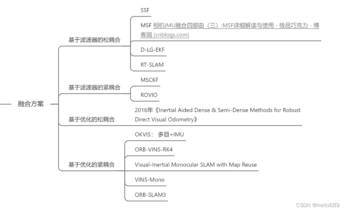
2020年推出的ORB-SLAM3方案,Binocular is provided+IMU的融合方案,并且ORB-SLAM3It was also introduced in the Deep Blue Academy Open Class.
工业界应用
VIOMainly the application of autonomous driving andAR、VR领域;比如可以使用手机进行AR换鞋(京东淘宝上有些店铺是支持AR试鞋的).以硬件为主打的XR头盔设备,目前在工业领域都一些落地的场景,如西门子的AR头盔的工业展示,飞机驾驶员的培训.
在学术界,VIO 研究有哪些新进展?有没有将学习方法用到VIO中的例子?
目前VIO和其他传感器的融合也是一个比较受欢迎的研究热点,比如VIO和激光雷达的融合,和GPS的融合.
- 2019, RAL, Visual-Inertial Localization with Prior LiDAR Map Constraints --视觉 VIO 和激光地图.
- 2018, arxiv, A General Optimization-based Framework for Global Pose Estimation with Multiple Sensors --VINS-Mono 的扩展版,能 融合 GPS、单目、双目等信息.
- 2017, ICRA, Vins on wheels --系统分析了 VIO + 轮速计系统的可观性.
- 2019, ICRA, Visual-Odometric Localization and Mapping for Ground Vehicles Using SE(2)-XYZ Constraints --SE2-XYZ 的模型来对地 面Wheel speed robot进行参数化.
VIO+深度学习
- VINet : Visual-inertial odometry as a sequence-to-sequence learning problem.就整体而言,VINet是首次使用DL的框架来解决VIO问题,目前所披露的实验表现出了一定的实用价值.
- Unsupervised Deep Visual-Inertial Odometry with Online Error Correction for RGB-D Imagery.此方法可以在没有Camera-IMU外参的情况下基于学习进行VIO网络学习整合IMU测量并生成估计轨迹,然后根据相对于像素坐标的空间网格的缩放图像投影误差的雅可比行列式在线校正.
参考博客:视觉惯性里程计 综述
题目:A review of visual inertial odometry from filtering and optimisation perspectives
期刊:Advanced Robotics | Volume 29,2015 - Issue 20
Author and research institution information:![[外链图片转存失败,源站可能有防盗链机制,建议将图片保存下来直接上传(img-Y1C2g4qd-1639382743957)(imgs/image-20211209201351549.png)]](/img/a4/0f074e41388fe7cd2d02158cfdc02d.png)
翻译:VIO综述论文
二、四元数和李代数更新
课件提到了可以使用四元数或旋转矩阵存储旋转变量.当我们用计算出来的 ω \omega ω对某旋转更新时,有两种不同方式:
R ← R exp ( ω ∧ ) 或 q ← q ⊗ [ 1 , 1 2 ω ] T R \leftarrow R \exp(\omega^{\wedge})\\ 或 q\leftarrow q \otimes [1, \frac{1}{2}\omega]^{T} R←Rexp(ω∧)或q←q⊗[1,21ω]T
请编程验证对于小量 ω \omega ω = [0.01, 0.02, 0.03]T,两种方法得到的结果非常接近,实践当中可视为等同.因此,在后文提到旋转时,我们并不刻意区分旋转本身是q 还是R,也不区分其更新方式为上式的哪一种.
代码编写
Program according to the formula,Refer to the textbookp48和p87页代码中对于eigen库和sophus库的使用.
The rotation vector refers to the example in the textbook,Set it to Edgez轴旋转45度.Use the rotation matrix to construct the corresponding quaternion,利用 Sophus::SO3d::hatThe antisymmetric matrix of the rotation vector can be found.
具体代码如下:
int main()
{
    //旋转矩阵
    Matrix3d rotation_matrix = Matrix3d::Identity();
    AngleAxisd rotation_vector(M_PI/4, Vector3d(0,0,1));  //表示沿Z轴旋转45度
    rotation_matrix = rotation_vector.toRotationMatrix();

    cout<<"R: "<<endl<<rotation_matrix<<endl<<endl;

    //Constructs the corresponding quaternion
    Eigen::Quaterniond q(rotation_matrix);
    cout << "q :"<< endl << q.coeffs().transpose() <<endl<<endl;

    //使用对数映射获得它的李代数
    Sophus::SO3d SO3_R(rotation_matrix);
    cout << "so3 :"<< endl << SO3_R.log().transpose() <<endl<<endl;

    //更新量omega
    Eigen::Vector3d omega(0.01, 0.02, 0.03); //更新量

    // 李代数更新
    Matrix3d skew_symmetric_matrix = Sophus::SO3d::hat(omega).matrix();
    cout<<"SO3 hat= "<<endl<< skew_symmetric_matrix<<endl<<endl;
    Sophus::SO3d SO3_updated = SO3_R * Sophus::SO3d::exp(omega);
    cout<<"SO3 updated = "<<endl<<(SO3_R * Sophus::SO3d::exp(omega)).matrix()<<endl<<endl;

    // 四元数更新
    Eigen::Quaterniond q_update(1, omega(0)/2, omega(1)/2, omega(2)/2);
    Eigen::Quaterniond q_updated = q * q_update.normalized();
    cout<<"Quaterniond updated = "<< endl << q_updated.toRotationMatrix() <<endl<<endl;

    //衡量两种方法之间的差距
    cout<<"disparity = "<< endl <<SO3_updated.matrix().transpose()*q_updated.toRotationMatrix()<<endl;
}
最终运行结果截图:
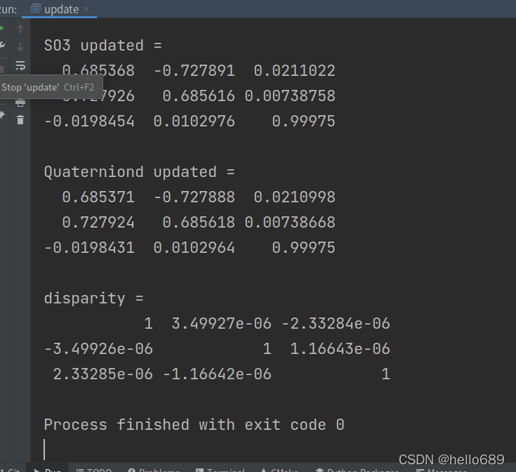
从实验结果可以看出,obtained in two different ways ω \omega ωThere is very little difference in the results of updating a certain rotation,(这里需要注意的一点是,Because the rotation matrix is on the Lie group,Lie groups do not have addition and subtraction,So the first one can be usedRThe inverse or transpose of the matrix is multiplied by the secondR矩阵,closer to the identity matrix,It means that the difference between the two matrices is smaller)差距在 1 0 − 6 10^{-6} 10−6以内,Therefore it is not deliberately distinguished that the rotation itself isq 还是R.
三、其他导数
使用右乘 s o ( 3 ) \mathfrak{so}(3) so(3),推导以下导数:
1.
d ( R − 1 p ) d R \frac{d(\mathbf{R}^{-1}p)}{d\mathbf{R}} dRd(R−1p)
右扰动:
d ( R − 1 p ) d R = d ( R − 1 p ) d φ = lim φ → 0 ( R exp ( φ ∧ ) ) − 1 p − R − 1 p φ = lim φ → 0 ( exp ( φ ∧ ) ) − 1 R − 1 p − R − 1 p φ = lim φ → 0 exp ( − φ ∧ ) R − 1 p − R − 1 p φ 泰 勒 展 开 ≈ lim φ → 0 ( I − φ ∧ ) R − 1 p − R − 1 p φ = lim φ → 0 − φ ∧ R − 1 p φ 根 据 s l a m 课 程 中 表 1 中 提 供 的 性 质 u ∧ v = − v ∧ u 可 得 : = lim φ → 0 ( R − 1 p ) ∧ φ φ = ( R − 1 p ) ∧ \begin{aligned} \frac{d(R^{-1} p)}{d R} &= \frac{d(R^{-1} p)}{d \varphi} \\ &= \lim\limits_{\varphi \to 0} \frac{(R \exp(\varphi^{\wedge}))^{-1}p-R^{-1}p}{\varphi} \\ &= \lim\limits_{\varphi \to 0} \frac{(\exp(\varphi^{\wedge}))^{-1}R^{-1}p-R^{-1}p}{\varphi} \\ &= \lim\limits_{\varphi \to 0} \frac{\exp(- \varphi^{\wedge})R^{-1}p-R^{-1}p}{\varphi} \\ 泰勒展开&\approx \lim\limits_{\varphi \to 0} \frac{(I- \varphi^{\wedge})R^{-1}p-R^{-1}p}{\varphi} \\&= \lim\limits_{\varphi \to 0} \frac{- \varphi^{\wedge}R^{-1}p}{\varphi} \\ 根据slamSchedule in the course1properties provided inu^{\wedge}v = -v^{\wedge}u可得: &= \lim\limits_{\varphi \to 0} \frac{(R^{-1}p)^{\wedge}\varphi}{\varphi} \\ &=(R^{-1}p)^{\wedge} \end{aligned} dRd(R−1p)泰勒展开根据slam课程中表1中提供的性质u∧v=−v∧u可得:=dφd(R−1p)=φ→0limφ(Rexp(φ∧))−1p−R−1p=φ→0limφ(exp(φ∧))−1R−1p−R−1p=φ→0limφexp(−φ∧)R−1p−R−1p≈φ→0limφ(I−φ∧)R−1p−R−1p=φ→0limφ−φ∧R−1p=φ→0limφ(R−1p)∧φ=(R−1p)∧
2.
d l n ( R 1 R 2 − 1 ) ∨ d R 2 \frac{d ln(\mathbf{R}_1\mathbf{R}_2^{-1})^{\vee}}{d\mathbf{R_2}} dR2dln(R1R2−1)∨
这里需要用BCHLinear approximation:
ln ( exp ( ϕ 1 ∧ ) exp ( ϕ 2 ∧ ) ) ∨ ≈ { J l ( ϕ 2 ) − 1 ϕ 1 + ϕ 2 当 ϕ 1 为 小 量 时 J r ( ϕ 1 ) − 1 ϕ 2 + ϕ 1 当 ϕ 2 为 小 量 时 \ln(\exp(\phi_1^{\wedge})\exp(\phi_2^{\wedge}))^{\vee} \approx \begin{cases} \mathcal{J}_l(\phi_2)^{-1}\phi_1 + \phi_2 &当\phi_1为小量时\\ \mathcal{J}_r(\phi_1)^{-1}\phi_2 + \phi_1 &当\phi_2为小量时 \end{cases} ln(exp(ϕ1∧)exp(ϕ2∧))∨≈{ Jl(ϕ2)−1ϕ1+ϕ2Jr(ϕ1)−1ϕ2+ϕ1当ϕ1为小量时当ϕ2为小量时
The following properties are also used:
( C u ) ∧ ≡ C u ∧ C T exp ( ( C u ) ∧ ) ≡ C exp ( u ∧ ) C T 旋 转 矩 阵 R − 1 = R T (\mathbf{C}u)^{\wedge}\equiv \mathbf{C}u^{\wedge}\mathbf{C}^T \\ \exp((\mathbf{C}u)^{\wedge}) \equiv \mathbf{C}\exp(u^{\wedge})\mathbf{C}^T \\ 旋转矩阵 R^{-1}=R^T (Cu)∧≡Cu∧CTexp((Cu)∧)≡Cexp(u∧)CT旋转矩阵R−1=RT
Calculate the above formula by means of right perturbation:
d ln ( R 1 R 2 − 1 ) ∨ d R 2 = lim φ 2 → 0 ln ( R 1 ( R 2 exp ( φ 2 ∧ ) ) − 1 ) ∨ − ln ( R 1 R 2 − 1 ) ∨ φ 2 = lim φ 2 → 0 ln ( R 1 exp ( − φ 2 ∧ ) R 2 − 1 ) ∨ − ln ( R 1 R 2 − 1 ) ∨ φ 2 = lim φ 2 → 0 ln ( R 1 R 2 − 1 R 2 exp ( − φ 2 ∧ ) R 2 T ) ∨ − ln ( R 1 R 2 − 1 ) ∨ φ 2 = lim φ 2 → 0 ln ( R 1 R 2 − 1 exp ( ( − R 2 φ 2 ) ∧ ) ) ∨ − ln ( R 1 R 2 − 1 ) ∨ φ 2 B C H 近 似 ≈ J r ( ln ( R 1 R 2 − 1 ) ∨ ) − 1 ( − R 2 φ 2 ) + ln ( R 1 R 2 − 1 ) ∨ − ln ( R 1 R 2 − 1 ) ∨ φ 2 = − J r ( ln ( R 1 R 2 − 1 ) ∨ ) − 1 ⋅ R 2 \begin{aligned} \frac{d \ln(R_1R_2^{-1})^{\vee}}{d R_2} &= \lim\limits_{\varphi_2 \to 0} \frac{\ln(R_1 (R_2 \exp(\varphi_2^{\wedge}))^{-1})^{\vee}-\ln(R_1 R_2^{-1})^{\vee}}{\varphi_2} \\&= \lim\limits_{\varphi_2 \to 0} \frac{\ln(R_1 \exp(-\varphi_2^{\wedge})R_2^{-1})^{\vee}-\ln(R_1 R_2^{-1})^{\vee}}{\varphi_2} \\&= \lim\limits_{\varphi_2 \to 0} \frac{\ln(R_1 R_2^{-1} R_2 \exp(-\varphi_2^{\wedge})R_2^T)^{\vee}-\ln(R_1 R_2^{-1})^{\vee}}{\varphi_2} \\&= \lim\limits_{\varphi_2 \to 0} \frac{\ln(R_1 R_2^{-1} \exp((-R_2\varphi_2)^{\wedge}))^{\vee}-\ln(R_1 R_2^{-1})^{\vee}}{\varphi_2} \\ BCH近似 &\approx \frac{\mathcal{J_r}(\ln(R_1R_2^{-1})^{\vee})^{-1}(-R_2\varphi_2) + \ln(R_1R_2^{-1})^{\vee}- \ln(R_1R_2^{-1})^{\vee}}{\varphi_2} \\ &= -\mathcal{J_r}(\ln(R_1R_2^{-1})^{\vee})^{-1} \cdot R_2 \end{aligned} dR2dln(R1R2−1)∨BCH近似=φ2→0limφ2ln(R1(R2exp(φ2∧))−1)∨−ln(R1R2−1)∨=φ2→0limφ2ln(R1exp(−φ2∧)R2−1)∨−ln(R1R2−1)∨=φ2→0limφ2ln(R1R2−1R2exp(−φ2∧)R2T)∨−ln(R1R2−1)∨=φ2→0limφ2ln(R1R2−1exp((−R2φ2)∧))∨−ln(R1R2−1)∨≈φ2Jr(ln(R1R2−1)∨)−1(−R2φ2)+ln(R1R2−1)∨−ln(R1R2−1)∨=−Jr(ln(R1R2−1)∨)−1⋅R2
代码地址:https://gitee.com/ximing689/vio-learning.git
边栏推荐
猜你喜欢
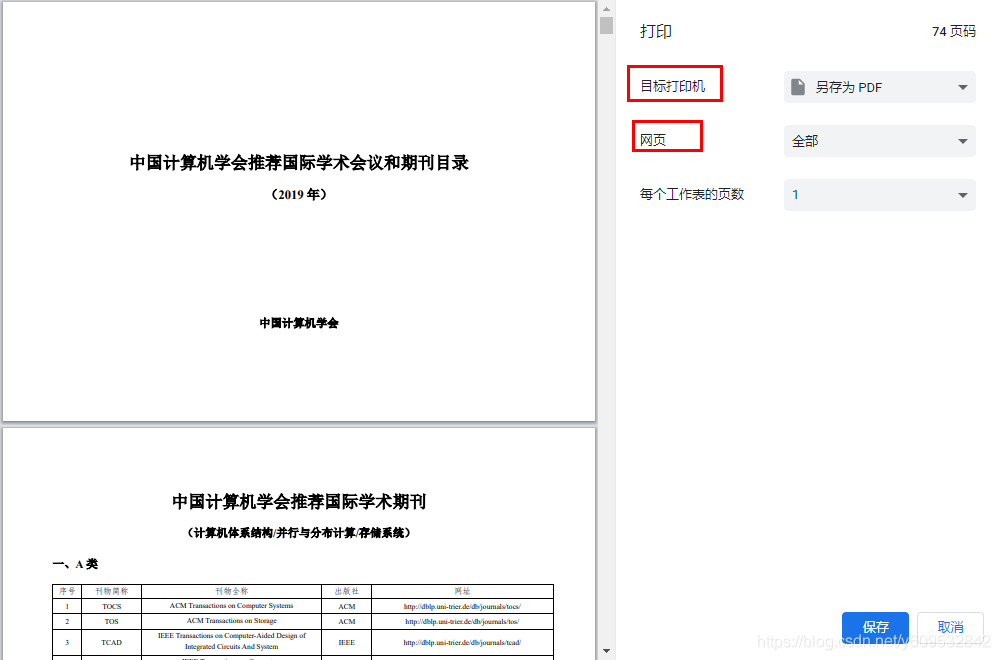
如何将PDF中的一部分页面另存为新的PDF文件

详解CAN总线:什么是CAN总线?

Deep Blue Academy - Visual SLAM Lecture Fourteen - Chapter 5 Homework
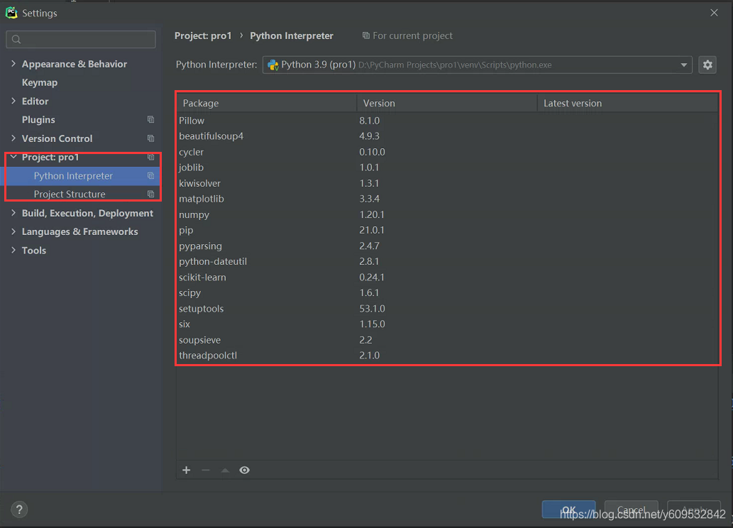
Pycharm平台导入scikit-learn
v-bind动态绑定
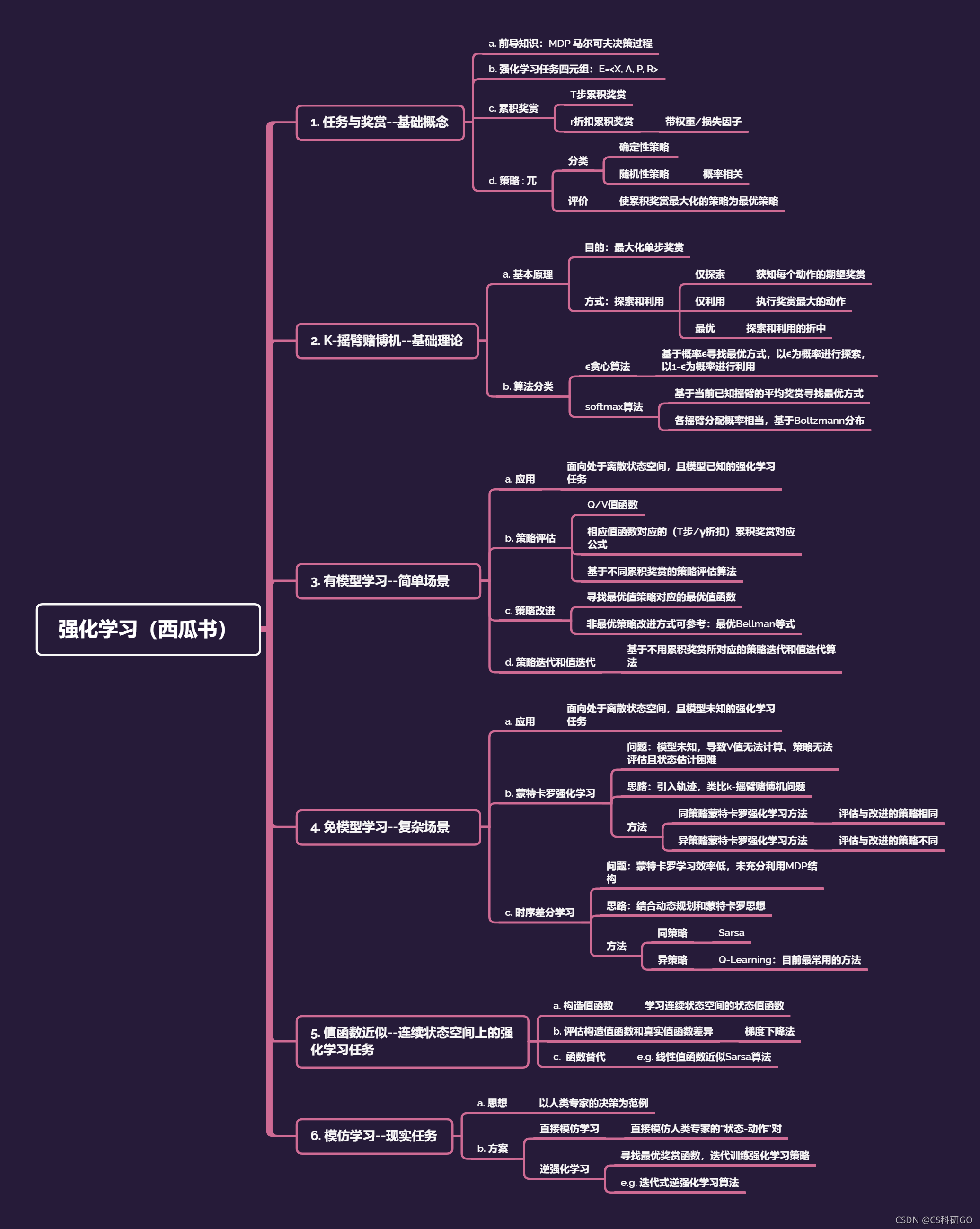
Reinforcement Learning (Chapter 16 of the Watermelon Book) Mind Map
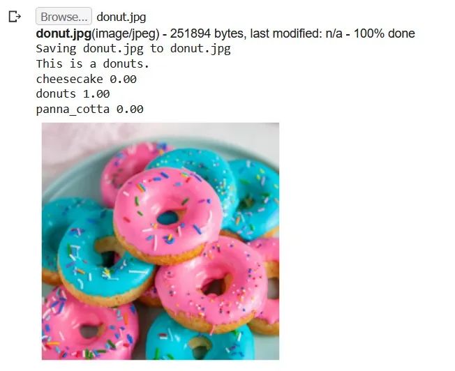
使用 Fastai 构建食物图像分类器
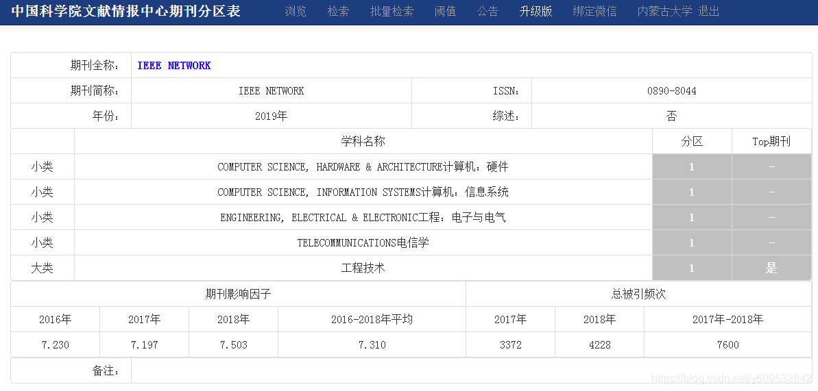
SCI期刊最权威的信息查询步骤!

吴恩达机器学习系列课程笔记——第八章:神经网络:表述(Neural Networks: Representation)

并发性,时间和相对性(1)-确定前后关系
随机推荐
多主复制的适用场景(1)-多IDC
深度剖析-class的几个对象(utlis,component)-瀑布流-懒加载(概念,作用,原理,实现步骤)
节流阀和本地存储
高等数学(第七版)同济大学 总习题三(后10题) 个人解答
吴恩达机器学习系列课程笔记——第十五章:异常检测(Anomaly Detection)
PHP5.6安装ssh2扩展用与执行远程命令
Nexus 5手机使用Nexmon工具获取CSI信息
v-bind动态绑定
ADSP21489工程中LDF文件配置详解
Zabbix删除一些大表历史数据脚本
ClickHouse的客户端命令行参数
OpenPCDet environment configuration of 3 d object detection and demo test
ScholarOne Manuscripts submits journal LaTeX file and cannot convert PDF successfully!
Research Notes (8) Deep Learning and Its Application in WiFi Human Perception (Part 1)
力扣 剑指 Offer 56 - I. 数组中数字出现的次数
吴恩达机器学习系列课程笔记——第六章:逻辑回归(Logistic Regression)
普氏分析法-MATLAB工具箱函数
深蓝学院-视觉SLAM十四讲-第六章作业
三维目标检测之OpenPCDet环境配置及demo测试
Win8.1下QT4.8集成开发环境的搭建