
print( "Hello,NumPy!" )
Learning is painful , Learn today , Lose tomorrow . This kind of weather , Or sleep is the most comfortable .

Let's talk about it , Make a noise , But you still have to learn .
In the process of learning, I always have the habit of taking notes , But the quality of the notes can't be flattered , Most of them have not been sorted out , But it's a good choice to review .
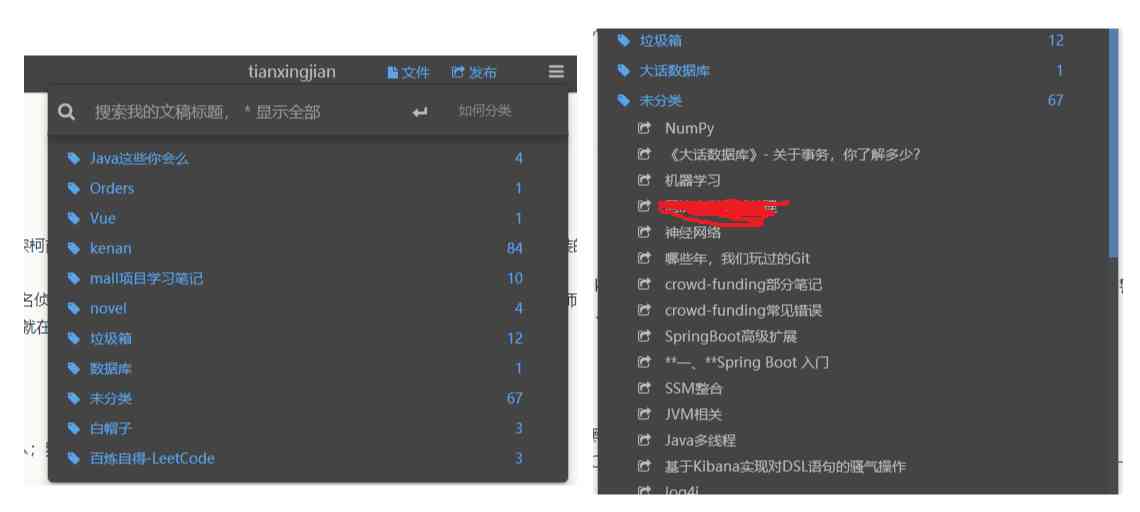
Self contact Python since , Most of them are reptiles , What kind of online novel , Virtual game currency , Examination question bank ah and so on have written , Also help others crawl a lot of website public data . I've collated an article about reptiles before ( Too lazy , Just one article , Then there's a chance to have time , Sort it out again ): Web crawler page style analysis
After that , That's right Social Engineering There was a certain interest , Maybe you need to be eloquent , have a glib tongue , achieve “ swindler ” Level of , Can we play social engineering . I wrote an article before Web Infiltrate relevant articles :Taoye Penetrate into a black platform headquarters , The truth behind it is terrible to think about it .
It is still necessary to remind you that , For someone or information that you don't trust , If you know something about cyber security , It can be used as a penetration experience , Otherwise , The best way to deal with it is to ignore , Don't let your curiosity be the beginning of the abyss , Especially in this cloud dragon hybrid virtual network world . Just a few days ago , The police also cracked the country's largest network luo liao What about extortion , Victim Da 10 More than ten thousand people , The amount involved is also XXXXXXXXXXXXXXX, We still need to pay attention to .
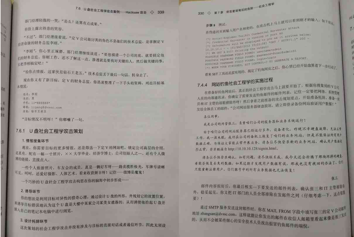
Anyway , There's a lot to learn 、 Very miscellaneous , I'm not good at learning , The notes are rarely reviewed . A good workman does his work well , You must sharpen your tools first , This doesn't start systematic learning, machine learning , So I want to put the previous record Numpy、Pandas、Matplotlib“ Three swordsmen ” Rearrange your notes , It's also a review .
Later on , Can learn some machine learning algorithms , Main reference 《 Machine learning practice / Machine Learning in Action》 With Mr. Zhou Zhihua 《 machine learning 》 Watermelon book , And some other technical articles written by some of the big guys in the circle . If you are good at it, try to tear it by hand , If you can't tear it by hand, it means that you still need to improve .
Flag Too many , I feel like I'll be slapped in the face . Don't worry , Take your time , I'm not afraid to fight in the face , Anyway, the skin is rough and the meat is thick ( ̄_, ̄ )
This article begins with NumPy Sort it out , Maybe it's not comprehensive , Only a few common ones are recorded , Other words will be used later to update it . The following content mainly refers to the rookie tutorial and NumPy Official documents :
- NumPy Novice tutorial :https://www.runoob.com/numpy/numpy-tutorial.html
- NumPy Official documents :https://numpy.org/doc/stable/user/quickstart.html
About NumPy Installation , I have already introduced the construction of deep learning environment , Recommended installation Anaconda, It integrates a large number of third-party tool modules , It doesn't have to be manual pip install ..., This is a bit like Java Medium Maven.Anaconda May refer to : be based on Ubuntu+Python+Tensorflow+Jupyter notebook Build a deep learning environment
If you have not installed Anaconda That's OK , Only need Python In the environment, execute the following command to install NumPy that will do :
> pip3 install numpy -i https://pypi.tuna.tsinghua.edu.cn/simple
The following is used in the following NumPy The version is :1.18.1
In [1]: import numpy as np

In [2]: np.__version__
Out[2]: '1.18.1'
stay NumPy in , The objects of operation are mostly ndarray type , It can also be called by another name array, We can think of it as a matrix or a vector .
establish np.ndarray Objects come in many ways ,NumPy There are also many api Available to call , For example, we can create a specified ndarray object :
In [7]: temp_array = np.array([[1, 2, 3], [4, 5, 6]], dtype = np.int32)

In [8]: temp_array
Out[8]:
array([[1, 2, 3],
       [4, 5, 6]])

In [9]: type(temp_array)
Out[9]: numpy.ndarray       #  The output is of type ndarray
Yes, of course , You can also call arange, And then it's done reshape Operation to change its shape , Convert a vector to 2x3 Matrix form of , The object type is still numpy.ndarray:
In [14]: temp_array = np.arange(1, 7).reshape(2, 3)     # arange Generating vectors ,reshape Change shape , Into a matrix

In [15]: temp_array
Out[15]:
array([[1, 2, 3],
       [4, 5, 6]])

In [16]: type(temp_array)       #  The type of output is still ndarray
Out[16]: numpy.ndarray
From above , We can find out , No matter what way ( Other methods will be introduced later ) To create objects ,NumPy It's all about ndarray type , And this type of object mainly contains the following properties :
- ndarray.ndim: Express ndarray The number of shaft , It can also be understood as dimension , Or it can be understood as the number of brackets in the outer layer . such as [1, 2, 3] Of ndim Namely 1,[[1], [2], [3]] Of ndim be equal to 2,[[[1]], [[2]], [[3]]] Of ndim be equal to 3( Pay attention to the number of brackets in the outer layer )
- ndarray.shape: Express ndarray The shape of the , The output is a tuple . The ndarray Yes n That's ok m Column , The output is (n, m), such as [[1], [2], [3]] The output is (3, 1),[[[1]], [[2]], [[3]]] The output is (3, 1, 1),[[[1, 2]], [[3, 4]]] The output is (2, 1, 2). Through the above 3 An example , You can find shape It is expressed from the outside to the inside
- ndarray.size: This is easier to understand , That means ndarray The total number of internal elements , That is to say shape The product of the
- ndarray.dtype: Express ndarray The data type of the internal element , Common are
numpy.int32、numpy.int64、numpy.float32、numpy.float64etc.
That's all ndarray Some of the common properties in , Be careful : Part of it , Not all of them , For other properties, please refer to the official documents
We can observe by the following ndarray Properties of , And how its internal properties should be modified :

In the above example np.expand_dims and np.astype It will be introduced later .
np.zeros You can create an element full of 0 Of ndarray,np.ones You can create an element full of 1 Of ndarray. You can specify ndarray Of shape shape , It can also be done through dtype Property specifies the data type of the inner element :
In [70]: np.zeros([2,3,2], dtype=np.float32)
Out[70]:
array([[[0., 0.],
        [0., 0.],
        [0., 0.]],

       [[0., 0.],
        [0., 0.],
        [0., 0.]]], dtype=float32)

In [71]: np.ones([3,2,2], dtype=np.float32)
Out[71]:
array([[[1., 1.],
        [1., 1.]],

       [[1., 1.],
        [1., 1.]],

       [[1., 1.],
        [1., 1.]]], dtype=float32)
in addition , stay Tensorflow Through tf.fill To generate a specified element shape tensor , As follows 2x3 Tensor , And the internal elements are 100:
In [76]: import tensorflow as tf

In [77]: tf.fill([2,3], 100)
Out[77]:
<tf.Tensor: shape=(2, 3), dtype=int32, numpy=
array([[100, 100, 100],
       [100, 100, 100]])>
And in the NumPy in , Also have fill Interface , It's just that you can only go through what you already have ndarray To call fill, Not directly np.fill To call :
In [79]: data = np.zeros([2, 3])

In [80]: data.fill(100)

In [81]: data
Out[81]:
array([[100., 100., 100.],
       [100., 100., 100.]])
np.arange With the usual range Works in a similar way , Used to produce a continuous interval ndarray, Pay attention to the left, not the right , And the array is an arithmetic sequence , Tolerances can be self-defined ( It can be a decimal ), as follows :
In [85]: np.arange(10)
Out[85]: array([0, 1, 2, 3, 4, 5, 6, 7, 8, 9])

In [86]: np.arange(3, 10, 2)
Out[86]: array([3, 5, 7, 9])

In [87]: np.arange(3, 10, 0.7)
Out[87]: array([3. , 3.7, 4.4, 5.1, 5.8, 6.5, 7.2, 7.9, 8.6, 9.3])
numpy.linspace Function to create a one-dimensional array , An array is made up of a sequence of equal differences , You can specify the number of elements inside the element and whether it contains stop value . as follows , In the interval 1-5 Create an element with the number of 10 Equal difference sequence of :
In [89]: np.linspace(1, 5, 10)      #  Default includes stop
Out[89]:
array([1.        , 1.44444444, 1.88888889, 2.33333333, 2.77777778,
       3.22222222, 3.66666667, 4.11111111, 4.55555556, 5.        ])

In [90]: np.linspace(1, 5, 10, endpoint = False)    # endpoint Property can be set to not contain stop
Out[90]: array([1. , 1.4, 1.8, 2.2, 2.6, 3. , 3.4, 3.8, 4.2, 4.6])
np.random.random and np.random.rand Random from 0-1 Generate corresponding to shape Of ndarray object :
In [4]: np.random.random([3, 2])
Out[4]:
array([[0.68755531, 0.56727707],
       [0.86027161, 0.01362836],
       [0.56557302, 0.94283249]])

In [5]: np.random.rand(2, 3)
Out[5]:
array([[0.19894754, 0.8568503 , 0.35165264],
       [0.75464769, 0.29596171, 0.88393648]])
np.random.randint Randomly generate a specified range of ndarray, And the internal elements are int type :
In [6]: np.random.randint(0, 10, [2, 3])
Out[6]:
array([[0, 6, 9],
       [5, 9, 1]])
np.random.randn Returns the standard normal distribution ndarray( The mean for 0, The variance of 1):
In [7]: np.random.randn(2,3)
Out[7]:
array([[ 2.46765106, -1.50832149,  0.62060066],
       [-1.04513254, -0.79800882,  1.98508459]])
in addition , We are NumPy Use in random When , It's a random set of data , and If you want to generate the same data each time , You have to go through np.random.seed To set it up :
In [33]: np.random.seed(100)

In [34]: np.random.randn(2, 3)
Out[34]:
array([[-1.74976547,  0.3426804 ,  1.1530358 ],
       [-0.25243604,  0.98132079,  0.51421884]])

In [35]: np.random.seed(100)

In [36]: np.random.randn(2, 3)
Out[36]:
array([[-1.74976547,  0.3426804 ,  1.1530358 ],
       [-0.25243604,  0.98132079,  0.51421884]])
stay NumPy One dimension in ndarray in , It's like a list , It can be sliced and traversed :
In [5]: a
Out[5]: array([1., 2., 3., 4., 5., 6., 7., 8., 9.])

In [6]: a[2], a[2:5]
Out[6]: (3.0, array([3., 4., 5.]))

In [7]: a * 3, a ** 3   #  cube
Out[7]:
(array([ 3.,  6.,  9., 12., 15., 18., 21., 24., 27.]),
 array([  1.,   8.,  27.,  64., 125., 216., 343., 512., 729.]))

In [13]: for i in a:
...:     print(i, end=", ")
1.0, 2.0, 3.0, 4.0, 5.0, 6.0, 7.0, 8.0, 9.0,
If our ndarray It's not a one-dimensional array , It's a two-dimensional matrix , Or higher dimensional ndarray, Then we need to segment it from multiple dimensions . And When we're dealing with high dimensional ndarray When traversing , The dimension of a single result is less than that of meta dimension , such as 2 The result of traversing dimensional matrix is 1 Dimension vector , The result of three-dimensional traversal is 2 D matrix .
in addition , There is one more thing to be said , The dimensions of my data are quite high , In order to facilitate us to index the data ,NumPy For us ... To segment , Specific examples are as follows :
In [14]: a = np.random.randint(0, 2, 6).reshape(2, 3)

In [15]: a
Out[15]:
array([[1, 1, 1],
       [1, 0, 1]])

In [16]: a[:, :2]
Out[16]:
array([[1, 1],
       [1, 0]])

In [17]: for i in a:        #  Traverse the matrix , Then the output is the row vector , A single output has fewer dimensions than the original 1
    ...:     print(i, end=", ")
[1 1 1], [1 0 1],

In [19]: data = np.random.randint(0, 2, [2, 2, 3])

In [20]: data
Out[20]:
array([[[0, 0, 1],
        [0, 1, 1]],

       [[1, 0, 0],
        [0, 1, 0]]])

In [21]: data[..., :2]      # ... It means that the first two dimensions need to be , amount to  data[:, :, :2]
Out[21]:
array([[[0, 0],
        [0, 1]],

       [[1, 0],
        [0, 1]]])
shape operation :
- a.ravel()、ndarray.flatten(), take ndarray Do the stretching operation ( Straighten it into vector form )
- a.reshape(), Re change a Of shape shape
- a.T、a.transpose(), return a The inverse matrix of
All of the above operations return new results , Without changing the original ndarray(a). And The above operations are all horizontal operations by default , If you need vertical , You need to control order Parameters , Specific operation can refer to rookie tutorial . except reshape outside , also resize, It's just resize Will change a Result , Instead of producing a new result :
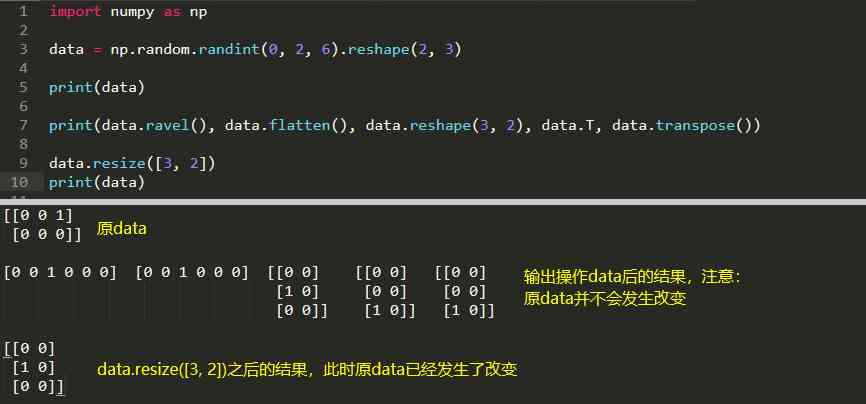
Another little trick to master is , It's going on reshape When , If it comes in -1, The corresponding result will be calculated automatically . For example, a 2x3 Matrix a, We carry out a.reshape(3, -1), And here it is -1 It stands for 2, When we have a lot of data , This is very convenient to use :
In [44]: a
Out[44]:
array([[1, 1, 1],
       [1, 0, 1]])

In [45]: a.reshape([3, -1])
Out[45]:
array([[1, 1],
       [1, 1],
       [0, 1]])
Modification of array dimensions :
| dimension | describe |
|---|---|
| broadcast_to | Broadcast array to new shape |
| expand_dims | Expand the shape of the array |
| squeeze | Remove one-dimensional entries from the shape of the array |
The specific operation is as follows :
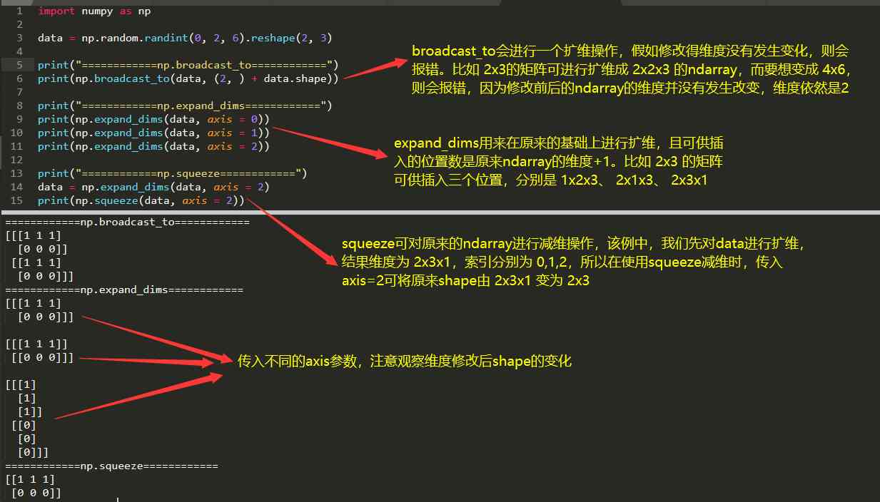
Array connection :
| function | describe |
|---|---|
| concatenate | Join the array sequence along the existing axis |
| hstack | Stack arrays in a sequence horizontally ( Column direction ) |
| vstack | Stack arrays in a sequence vertically ( Line direction ) |
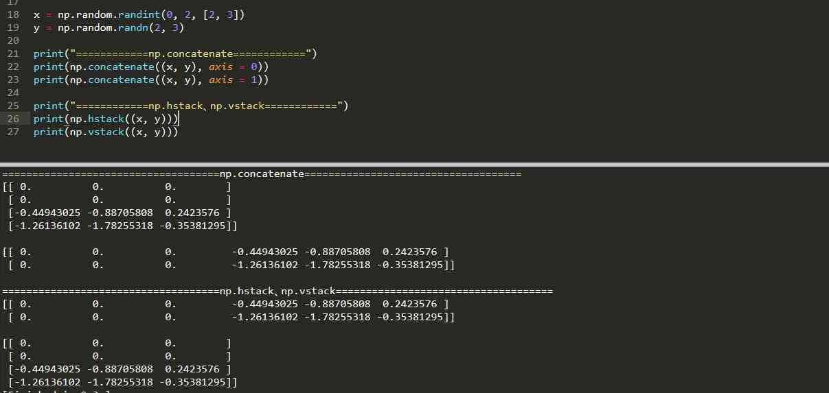
The following code shows the operation of array join , among concatenate By controlling axis To determine the direction of the connection , The effect is equal to hstack and vstack. Another thing to note is : The following example simply concatenates two arrays , In fact, you can connect multiple , such as np.concatenate((x, y, z), axis=1)
Segmentation of arrays :
| function | describe |
|---|---|
| split | Divide an array into multiple subarrays |
| hsplit | Divide an array horizontally into multiple subarrays ( By column ) |
| vsplit | Divide an array vertically into multiple subarrays ( Press the line ) |
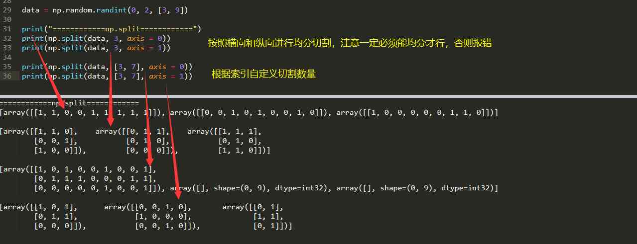
It's the same as an array join ,split By controlling axis Property to get the same as hsplit、vsplit Same effect , Here's just split An example of , About hsplit and vsplit Refer to official documents :
Addition and deletion of array elements :
| function | describe |
|---|---|
| append | Add values to the end of the array |
| insert | Inserts a value along the specified axis before the specified subscript |
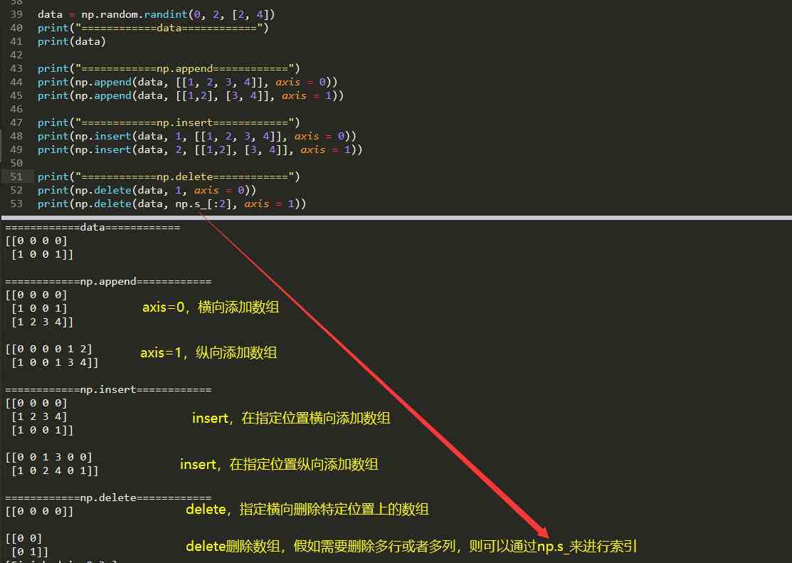
| delete | Delete the subarray of a certain axis , And return the new array after deletion |
radio broadcast (Broadcast) yes numpy For different shapes (shape) How to do the numerical calculation of the array , Arithmetic operations on arrays are usually performed on the corresponding elements .
If two arrays a and b The same shape , The meet a.shape == b.shape, that a*b The result is that a And b Array corresponding bit multiplication . This requires the same dimension , And the length of each dimension is the same .
In [8]: import numpy as np

In [9]: a = np.array([1,2,3,4])
   ...: b = np.array([10,20,30,40])

In [10]: a * b
Out[10]: array([ 10,  40,  90, 160])
When in operation 2 The shapes of arrays are different ,numpy Will automatically trigger the broadcast mechanism . Such as :
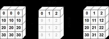
In [11]: a = np.array([[ 0, 0, 0],
    ...:            [10,10,10],
    ...:            [20,20,20],
    ...:            [30,30,30]])
    ...: b = np.array([1,2,3])

In [12]: a + b
Out[12]:
array([[ 1,  2,  3],
       [11, 12, 13],
       [21, 22, 23],
       [31, 32, 33]])
The following image shows the array b How to broadcast with array a compatible .
np.tile It can broadcast the target operation array , such as 1x3 The following operations can be broadcast as 4x6, Pay attention to the above broadcast_to Make a difference ,broadcast_to It has to be expanded , and tile Extendable dimension , We can not expand the dimension , Specific operation according to their own actual needs .
There was Tensorflow Experienced readers should know , It also has tile and broadcast operation , But when we have a large amount of data , It is said that tile Is more efficient than broadcast Be low , I don't know why , It will be useful in the future .
In [20]: a
Out[20]: array([[1, 1, 0]])

In [21]: np.tile(a, [4, 2])     #  The second parameter represents the multiple of each dimension broadcast , This is line expansion 4 times , Liege 2 times
Out[21]:
array([[1, 1, 0, 1, 1, 0],
       [1, 1, 0, 1, 1, 0],
       [1, 1, 0, 1, 1, 0],
       [1, 1, 0, 1, 1, 0]])
About NumPy Copy and attempt in : This part of the knowledge is also what I was learning before NumPy The missing points of time , Take advantage of this opportunity , Record it here .
- No copy
On this point , Actually, it was recorded before LeetCode Hot topic HOT 100(01, Addition of two numbers ) The algorithm also mentioned , This point needs to be paid more attention to .
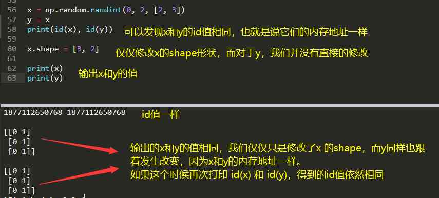
- View or shallow copy (view)
Use the same code as above , Only the... Has been modified 57 That's ok , take y = x and y = x.view(), You can find , At this time x and y Of id Values are not the same , They don't have the same memory address , We modify x Of shape after ,y Of shape Nothing has changed .
however , When we change, it's not shape, Instead, change the data inside a variable array , The other array changes as well

- Copy or deep copy (copy)
The view or shallow copy uses view, And copy or deep copy uses copy. Use copy When modifying an array shape, Or internal elements , The other array doesn't change .
( About copy, The code is no longer demonstrated here , Readers can operate by themselves , And then compare them )
So to conclude :
- y = x, explain x and y Of Same memory address , Modify one of , The other will change as it happens ( Whether it's shape, Or internal elements )
- y = x.view(), The memory addresses of the two are different , Modify one of the shape, The other doesn't change ; And modify the inner elements of one of the tuples , The other one will change with it
- y = x.copy(), The memory addresses of the two are different , Whether it's modifying a tuple shape, Or internal elements , None of the other will change , They are independent of each other
NumPy The mathematical correlation function in , There is nothing to talk about in this part :
- np.pi, return π value
- np.sin(), Return sine value
- np.cos(), Returns the cosine of
- np.tan(), Return tangent value
- numpy.ceil(), Returns the smallest integer greater than or equal to the specified expression , That is, round up .
- np.exp(2), Returns the index value , That is to say $e^2$
Other related mathematical functions , Refer to official documents .
NumPy The arithmetic operations in , There is nothing to talk about in this part :
- numpy.add(a,b): Add two arrays
- numpy.subtract(a,b): Subtracting two arrays
- numpy.multiply(a,b): Multiply two arrays
- numpy.divide(a,b): Divide two arrays by
- numpy.reciprocal(a), Back to the bottom
- numpy.power(a, 4), return a The fourth power of
NumPy The statistical function in , This is a little bit of a note :
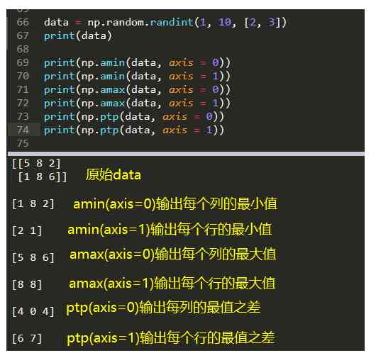
The above example shows how to get the maximum value and the difference between the maximum value and the maximum value in an array , Into axis Parameters , Then we get it in the corresponding direction , If there is no introduction axis Parameters , It means to get the maximum value of the whole array . In addition to the above interfaces , There are other common statistical functions , There is no difference between the specific operation and the above , as follows :
- np.amin(): Get the minimum
- np.amax(): Get the maximum
- np.ptp(): Get the difference between the maximum and the minimum
- np.median(): Get the median ( The median )
- np.mean(): Get the mean
- np.var(): To obtain the variance ,$\sigma^2 = \frac{1}{n}\sum_{i=1}n(x_i-\overline{x})2$
- np.std(): Get the standard deviation ,$\sigma$
NumPy Linear algebra in :
- np.dot(a, b) It's the product of two matrices
- np.vdot(a, b) The sum of the products of the corresponding positions of two matrices
- np.inner(a, b) Inner product , Namely a With each line of b Each line of the sum
such as a=[[1, 0], [1, 1]],b=[[1, 2], [1, 3]]
np.inner(a, b) amount to [1, 0] * [1, 2] = 1 -> For the first number
[1, 0] * [1, 3] = 1 -> For the second number
[1, 1] * [1, 2] = 3 -> For the third number
[1, 1] * [1, 3] = 4 -> For the fourth number
The matrix product is the sum of the product of the row of the first matrix and the column product of the second matrix , and inner It is equivalent to the sum of the row products of the first matrix and the second matrix
- np.matmul(a, b) Feeling and np.dot(a, b) It works the same , They're all matrix products
- np.linalg.det(a) Calculate the value of the determinant of a matrix
- np.linalg.solve(a, [[1], [1]]) Find solutions to linear equations , The first parameter corresponds to the coefficient , The second parameter is equivalent to the parameter term
- np.linalg.inv(a) Calculate the inverse of a matrix
#  Save the array to  .npy  In the file with the extension .
numpy.save(file, arr, allow_pickle=True, fix_imports=True)
- file: File to save , extension .npy, If there is no extension at the end of the file path .npy, The extension will be automatically added with .
- arr: The array to save
- allow_pickle: Optional , Boolean value , Allow to use Python pickles Save an array of objects ,Python Medium pickle Used before saving to or reading from a disk file , Serialize and deserialize objects .
- fix_imports: Optional , For convenience Pyhton2 Read from Python3 Saved data .
In [81]: a = np.random.randint(1, 10, [3, 4])

In [82]: np.save("a.npy", a)

In [83]: np.load("a.npy")
Out[83]:
array([[2, 7, 3, 1],
       [4, 6, 4, 3],
       [2, 2, 9, 5]])
Reference material :
Reference material :
[1] NumPy Novice tutorial :https://www.runoob.com/numpy/numpy-tutorial.html
[2] NumPy Official documents :https://numpy.org/doc/stable/user/quickstart.html
Not enough time , It's a bit hasty to write later , But should not affect the normal reading and later review , For the time being .
Be careful : Only a few common ones are recorded , Other words will be used later to update it , Other contents can refer to the document .
It was meant to be in accordance with 《 Machine learning practice / Machine Learning in Action》 This book is about to tear the code out of it , But for practical reasons , It may need to be torn by hand SVM 了 , This algorithm is still a headache , It's too complicated inside , There are few data to deduce it completely , It also involves a lot of nouns of "Mo Sheng" , Such as : Optimization under nonlinear constraints 、KKT Conditions 、 Lagrange dual 、 The largest interval 、 The optimal lower bound 、 Kernel functions and so on , The book of heaven may be 、 Probably 、 Maybe that's it . Fortunately, I have studied before SVM, But it must still take a lot of energy to tear , Also need to refer to a lot of information , Including but not limited to 《 Machine learning practice / Machine Learning in Action》、《 machine learning 》、《 Statistical learning method 》.
therefore , In the next issue , It should start tearing SVM, As for whether we can succeed in the end , It's hard to say . It may take a lot of time , During this period LeetCode HOT 100 And it needs to be painted normally .
I am a Taoye, Love to study , Love sharing , Keen on all kinds of Technology , I like playing chess in my spare time 、 Listen to the music 、 Talking about animation , I hope to take this opportunity to record my growth process and life , Also hope to be able to foster more like-minded friends in the circle , For more information, welcome to wechat Princess : Cynical Coder.
Recommended reading :
Why not , Eat first
Taoye Penetrate into a black platform headquarters , The truth behind it is terrible to think about it
《 Big talk database 》-SQL Statement execution time , What little action did the bottom layer do ?
In those years , We played Git, It's delicious
be based on Ubuntu+Python+Tensorflow+Jupyter notebook Build a deep learning environment
Web crawler page style analysis
A handshake will help you understand Docker Container technology
A detailed explanation Hexo+Github Xiaobai builds a station
open ElasticSearch、kibana、logstash The right way

