Opencv Learning Notes 6 -- image feature [harris+sift]+ feature matching

Image features （SIFT-Scale Invariant Feature Transform）

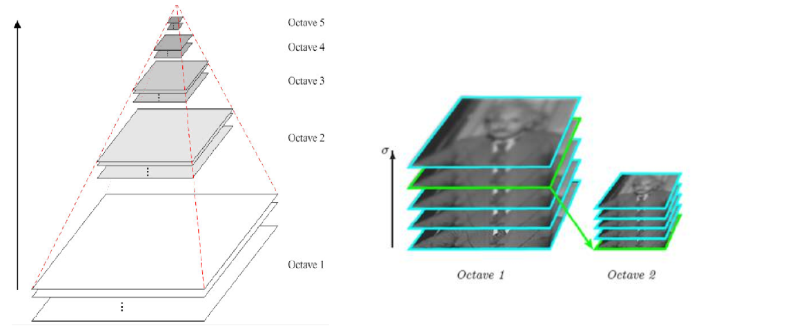
Image scale space

To a certain extent , Whether the object is big or small , The human eye can tell , But it's hard for computers to have the same capabilities , So let the machine be able to have a unified understanding of objects at different scales , We need to consider the characteristics of images in different scales .

The scale space is usually obtained by Gaussian blur

Different σ The Gaussian function determines the smoothness of the image , The bigger σ The more blurred the image is .

Multiresolution pyramid

Gaussian difference pyramid （DOG）

DoG Spatial extremum detection

In order to find the extremum of scale space , Each pixel and its image domain （ The same scale space ） And scale domain （ Adjacent scale space ） Compare all the adjacent points of , When it is greater than （ Or less than ） At all adjacent points , This point is the extreme point . As shown in the figure below , In the middle of the detection point and its image of 3×3 Neighborhood 8 Pixels , And its adjacent upper and lower floors 3×3 field 18 Pixels , common 26 Compare pixels .

Precise positioning of key points

The key points of these candidates are DOG The local extremum of a space , And these extreme points are discrete points , One way to accurately locate the extreme point is , For scale space DoG Function for curve fitting , Calculate its extreme point , So as to realize the precise positioning of key points .

Eliminate boundary response

The main direction of the feature point

Each feature point can get three information (x,y,σ,θ), I.e. location 、 Scale and direction . Keys with multiple directions can be copied into multiple copies , Then the direction values are assigned to the copied feature points respectively , A feature point produces multiple coordinates 、 The scales are equal , But in different directions .

Generating feature descriptions

After finishing the gradient calculation of the key points , Use histogram to count the gradient and direction of pixels in the neighborhood .

In order to ensure the rotation invariance of the feature vector , Focus on feature points , Rotate the axis in the neighborhood θ angle , That is, the coordinate axis is rotated to the main direction of the feature point .

The main direction after rotation is the center 8x8 The window of , Find the gradient amplitude and direction of each pixel , The direction of the arrow represents the direction of the gradient , The length represents the gradient amplitude , Then the Gaussian window is used to weight it , At the end of each 4x4 Draw on a small piece of 8 Gradient histogram in three directions , Calculate the cumulative value of each gradient direction , A seed point can be formed , That is, each feature is represented by 4 It is composed of seed points , Each seed point has 8 Vector information in three directions .

It is suggested that each key point should be used 4x4 common 16 A seed point to describe , Such a key point will produce 128 Dimensional SIFT Eigenvector .

opencv SIFT function

import cv2
import numpy as np
import matplotlib.pyplot as plt#Matplotlib yes RGB

img = cv2.imread('test_1.jpg')
gray = cv2.cvtColor(img, cv2.COLOR_BGR2GRAY)

def cv_show(img,name):
    b,g,r = cv2.split(img)
    img_rgb = cv2.merge((r,g,b))
    plt.imshow(img_rgb)
    plt.show()
def cv_show1(img,name):
    plt.imshow(img)
    plt.show()
    cv2.imshow(name,img)
    cv2.waitKey()
    cv2.destroyAllWindows()

cv2.__version__ #3.4.1.15 pip install opencv-python==3.4.1.15 pip install opencv-contrib-python==3.4.1.15

'3.4.1'

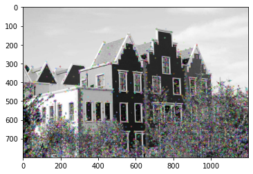
Get the feature point

sift = cv2.xfeatures2d.SIFT_create()
kp = sift.detect(gray, None)

img = cv2.drawKeypoints(gray, kp, img)
cv_show(img,'drawKeypoints')
# cv2.imshow('drawKeypoints', img)
# cv2.waitKey(0)
# cv2.destroyAllWindows()

Calculating characteristics

kp, des = sift.compute(gray, kp)

print (np.array(kp).shape)

(6827,)

des.shape

(6827, 128)

des[0]

array([  0.,   0.,   0.,   0.,   0.,   0.,   0.,   0.,  21.,   8.,   0.,
         0.,   0.,   0.,   0.,   0., 157.,  31.,   3.,   1.,   0.,   0.,
         2.,  63.,  75.,   7.,  20.,  35.,  31.,  74.,  23.,  66.,   0.,
         0.,   1.,   3.,   4.,   1.,   0.,   0.,  76.,  15.,  13.,  27.,
         8.,   1.,   0.,   2., 157., 112.,  50.,  31.,   2.,   0.,   0.,
         9.,  49.,  42., 157., 157.,  12.,   4.,   1.,   5.,   1.,  13.,
         7.,  12.,  41.,   5.,   0.,   0., 104.,   8.,   5.,  19.,  53.,
         5.,   1.,  21., 157.,  55.,  35.,  90.,  22.,   0.,   0.,  18.,
         3.,   6.,  68., 157.,  52.,   0.,   0.,   0.,   7.,  34.,  10.,
        10.,  11.,   0.,   2.,   6.,  44.,   9.,   4.,   7.,  19.,   5.,
        14.,  26.,  37.,  28.,  32.,  92.,  16.,   2.,   3.,   4.,   0.,
         0.,   6.,  92.,  23.,   0.,   0.,   0.], dtype=float32)

Image features -harris Corner detection

The basic principle

cv2.cornerHarris()

• img： The data type is float32 Into the image of
• blockSize： The size of the specified area in corner detection
• ksize： Sobel Window size used in derivation
• k： The value parameter is [0,04,0.06]

import cv2 
import numpy as np
import matplotlib.pyplot as plt#Matplotlib yes RGB

img = cv2.imread('chessboard.jpg')
print ('img.shape:',img.shape)
gray = cv2.cvtColor(img, cv2.COLOR_BGR2GRAY)
# gray = np.float32(gray)
dst = cv2.cornerHarris(gray, 2, 3, 0.04)
print ('dst.shape:',dst.shape)

img.shape: (512, 512, 3)
dst.shape: (512, 512)

def cv_show(img,name):
    b,g,r = cv2.split(img)
    img_rgb = cv2.merge((r,g,b))
    plt.imshow(img_rgb)
    plt.show()
def cv_show1(img,name):
    plt.imshow(img)
    plt.show()
    cv2.imshow(name,img)
    cv2.waitKey()
    cv2.destroyAllWindows()

img[dst>0.01*dst.max()]=[255,255,255]
cv_show(img,'dst')
# cv2.imshow('dst',img) 
# cv2.waitKey(0) 
# cv2.destroyAllWindows()

Feature matching

Brute-Force Brute force match

import cv2 
import numpy as np
import matplotlib.pyplot as plt
%matplotlib inline

img1 = cv2.imread('box.png', 0)
img2 = cv2.imread('box_in_scene.png', 0)

def cv_show(img,name):
    b,g,r = cv2.split(img)
    img_rgb = cv2.merge((r,g,b))
    plt.imshow(img_rgb)
    plt.show()
def cv_show1(img,name):
    plt.imshow(img)
    plt.show()
    cv2.imshow(name,img)
    cv2.waitKey()
    cv2.destroyAllWindows()

cv_show1(img1,'img1')

cv_show1(img2,'img2')

sift = cv2.xfeatures2d.SIFT_create()

kp1, des1 = sift.detectAndCompute(img1, None)
kp2, des2 = sift.detectAndCompute(img2, None)

# crossCheck It means that two feature points should match each other , for example A No i Characteristic points and B No j The nearest feature point , also B No j Feature points to A No i The feature points are also  
#NORM_L2:  Normalized array of ( Euclid distance ), If other feature calculation methods need to consider different matching calculation methods 
bf = cv2.BFMatcher(crossCheck=True) # Brute force match 

1 Yes 1 The matching of

matches = bf.match(des1, des2)
matches = sorted(matches, key=lambda x: x.distance)# Sort 

img3 = cv2.drawMatches(img1, kp1, img2, kp2, matches[:10], None,flags=2)

cv_show(img3,'img3')

k For the best match

bf = cv2.BFMatcher()
matches = bf.knnMatch(des1, des2, k=2)#1 Yes K matching  

good = []
for m, n in matches:
    if m.distance < 0.75 * n.distance:
        good.append([m])

img3 = cv2.drawMatchesKnn(img1,kp1,img2,kp2,good,None,flags=2)

cv_show(img3,'img3')

If you need to complete the operation more quickly , You can try to use cv2.FlannBasedMatcher

Random sampling consistency algorithm （Random sample consensus,RANSAC）

Select the initial sample points for fitting , Given a tolerance range , Keep iterating

After each fitting , There are corresponding data points within the tolerance range , Find out the situation with the largest number of data points , Is the final fitting result

Homography matrix