当前位置:网站首页>t-sne 数据可视化网络中的部分参数+
t-sne 数据可视化网络中的部分参数+
2022-07-31 15:29:00 【FakeOccupational】
注:本代码主要实现对于网络中对于某个中间特征或计算得到的网络参数的可视化实现。如果仅可视化网络中的某个简单的参数,可以考虑使用 model.weight得到矩阵,然后放入分部代码中的降维可视化部分即可。TSNE参数说明
总体代码
import torch
import torch.nn as nn
import torch.nn.functional as F
from sklearn.manifold import TSNE
import matplotlib.pyplot as plt


class Network(nn.Module):  # extend nn.Module class of nn
    def __init__(self):
        super().__init__()  # super class constructor
        self.conv1 = nn.Conv2d(in_channels=1, out_channels=6, kernel_size=(5, 5))
        self.batchN1 = nn.BatchNorm2d(num_features=6)
        self.conv2 = nn.Conv2d(in_channels=6, out_channels=12, kernel_size=(5, 5))
        self.fc1 = nn.Linear(in_features=12 * 4 * 4, out_features=120)
        self.batchN2 = nn.BatchNorm1d(num_features=120)
        self.fc2 = nn.Linear(in_features=120, out_features=60)
        self.out = nn.Linear(in_features=60, out_features=10)

    def forward(self, t):  # implements the forward method (flow of tensors)

        # hidden conv layer
        t = self.conv1(t)
        t = F.max_pool2d(input=t, kernel_size=2, stride=2)
        t = F.relu(t)
        t = self.batchN1(t)

        # hidden conv layer
        t = self.conv2(t)
        t = F.max_pool2d(input=t, kernel_size=2, stride=2)
        t = F.relu(t)

        # flatten
        t = t.reshape(-1, 12 * 4 * 4)
        t = self.fc1(t)
        t = F.relu(t)
        t = self.batchN2(t)
        t = self.fc2(t)
        t = F.relu(t)

        # output
        t = self.out(t)

        return t
cnn_model = Network() # init model


pretrained_dict = cnn_model.state_dict()


class Identity(nn.Module):
    def __init__(self):
        super(Identity, self).__init__()
        self.conv1 = nn.Conv2d(in_channels=1, out_channels=6, kernel_size=(5, 5))

    def forward(self, x):
        return x


model = Identity()
model_dict = model.state_dict()
# model.load_state_dict(pretrained_dict) # RuntimeError: Error(s) in loading state_dict for Identity: Unexpected key(s) in state_dict: "batchN1.weight", "batchN1.bias", "batchN1.running_mean",


# 1. filter out unnecessary keys
pretrained_dict = {
    k: v for k, v in pretrained_dict.items() if k in model_dict}
# 2. overwrite entries in the existing state dict
model_dict.update(pretrained_dict)
# 3. load the new state dict
model.load_state_dict(pretrained_dict)

vector = model.conv1.weight.detach().numpy()[0,0,:,:]

digits_final = TSNE(perplexity=30).fit_transform(vector)  #
plt.scatter(digits_final[:,0], digits_final[:,1])
plt.show()
功能分部代码
模型处理部分
import torch
import torch.nn as nn
import torch.nn.functional as F


class Network(nn.Module):  # extend nn.Module class of nn
    def __init__(self):
        super().__init__()  # super class constructor
        self.conv1 = nn.Conv2d(in_channels=1, out_channels=6, kernel_size=(5, 5))
        self.batchN1 = nn.BatchNorm2d(num_features=6)
        self.conv2 = nn.Conv2d(in_channels=6, out_channels=12, kernel_size=(5, 5))
        self.fc1 = nn.Linear(in_features=12 * 4 * 4, out_features=120)
        self.batchN2 = nn.BatchNorm1d(num_features=120)
        self.fc2 = nn.Linear(in_features=120, out_features=60)
        self.out = nn.Linear(in_features=60, out_features=10)

    def forward(self, t):  # implements the forward method (flow of tensors)

        # hidden conv layer
        t = self.conv1(t)
        t = F.max_pool2d(input=t, kernel_size=2, stride=2)
        t = F.relu(t)
        t = self.batchN1(t)

        # hidden conv layer
        t = self.conv2(t)
        t = F.max_pool2d(input=t, kernel_size=2, stride=2)
        t = F.relu(t)

        # flatten
        t = t.reshape(-1, 12 * 4 * 4)
        t = self.fc1(t)
        t = F.relu(t)
        t = self.batchN2(t)
        t = self.fc2(t)
        t = F.relu(t)

        # output
        t = self.out(t)

        return t
cnn_model = Network() # init model


pretrained_dict = cnn_model.state_dict()


class Identity(nn.Module):
    def __init__(self):
        super(Identity, self).__init__()
        self.conv1 = nn.Conv2d(in_channels=1, out_channels=6, kernel_size=(5, 5))

    def forward(self, x):
        return x


model = Identity()
model_dict = model.state_dict()
# model.load_state_dict(pretrained_dict) # RuntimeError: Error(s) in loading state_dict for Identity: Unexpected key(s) in state_dict: "batchN1.weight", "batchN1.bias", "batchN1.running_mean",


# 1. filter out unnecessary keys
pretrained_dict = {
    k: v for k, v in pretrained_dict.items() if k in model_dict}
# 2. overwrite entries in the existing state dict
model_dict.update(pretrained_dict)
# 3. load the new state dict
model.load_state_dict(pretrained_dict)
降维可视化部分
import numpy as np


import sklearn #Import scikitlearn for machine learning functionalities
from sklearn.manifold import TSNE
from sklearn.datasets import load_digits # For the UCI ML handwritten digits dataset

import matplotlib # Matplotlib 是 Python 中的一个库,它是 NumPy 库的数值数学扩展
import matplotlib.pyplot as plt
import matplotlib.patheffects as pe


import seaborn as sb


digits = load_digits()
print(digits.data.shape) # There are 10 classes (0 to 9) with alomst 180 images in each class
                         # The images are 8x8 and hence 64 pixels(dimensions)
plt.gray();
#Displaying what the standard images look like
for i in range(0,10):
    plt.matshow(digits.images[i])
    plt.show()


X = np.vstack([digits.data[digits.target==i] for i in range(10)]) # Place the arrays of data of each digit on top of each other and store in X
# X = np.random.random([1797, 64])

#Implementing the TSNE Function - ah Scikit learn makes it so easy!
digits_final = TSNE(perplexity=30).fit_transform(X) # plt.scatter(digits_final[0], digits_final[1])
#Play around with varying the parameters like perplexity, random_state to get different plots


# With the above line, our job is done. But why did we even reduce the dimensions in the first place?
# To visualise it on a graph.

# So, here is a utility function that helps to do a scatter plot of thee transformed data

def plot(x, colors):
    palette = np.array(sb.color_palette("hls", 10))  # Choosing color palette

    # Create a scatter plot.
    f = plt.figure(figsize=(8, 8))
    ax = plt.subplot(aspect='equal')
    sc = ax.scatter(x[:, 0], x[:, 1], lw=0, s=40, c=palette[colors.astype(np.int)])


    # 添加文本
    txts = []
    # for i in range(10):
    #     # Position of each label.
    # xtext, ytext = np.median(x[colors == i, :], axis=0) # 返回数组元素的中位数。
    # txt = ax.text(xtext, ytext, str(i), fontsize=24) # Text(6.610861, 37.19979, '9')
    # txt.set_path_effects([pe.Stroke(linewidth=5, foreground="w"), pe.Normal()])# 文本效果
    # txts.append(txt)
    return f, ax, txts


Y = np.hstack([digits.target[digits.target==i] for i in range(10)]) # Place the arrays of data of each target digit by the side of each other continuosly and store in Y
plot(digits_final,Y)
plt.show()
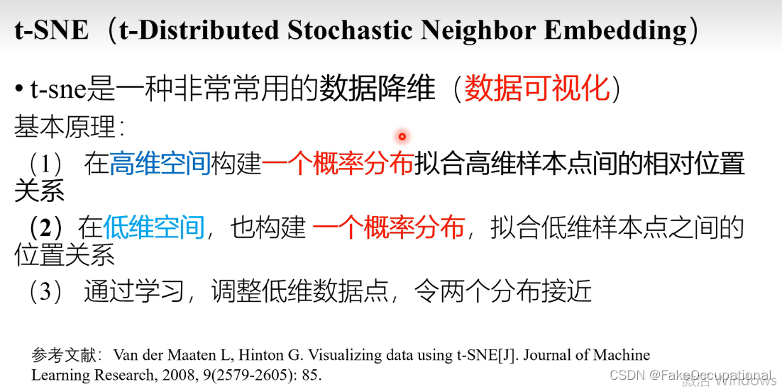
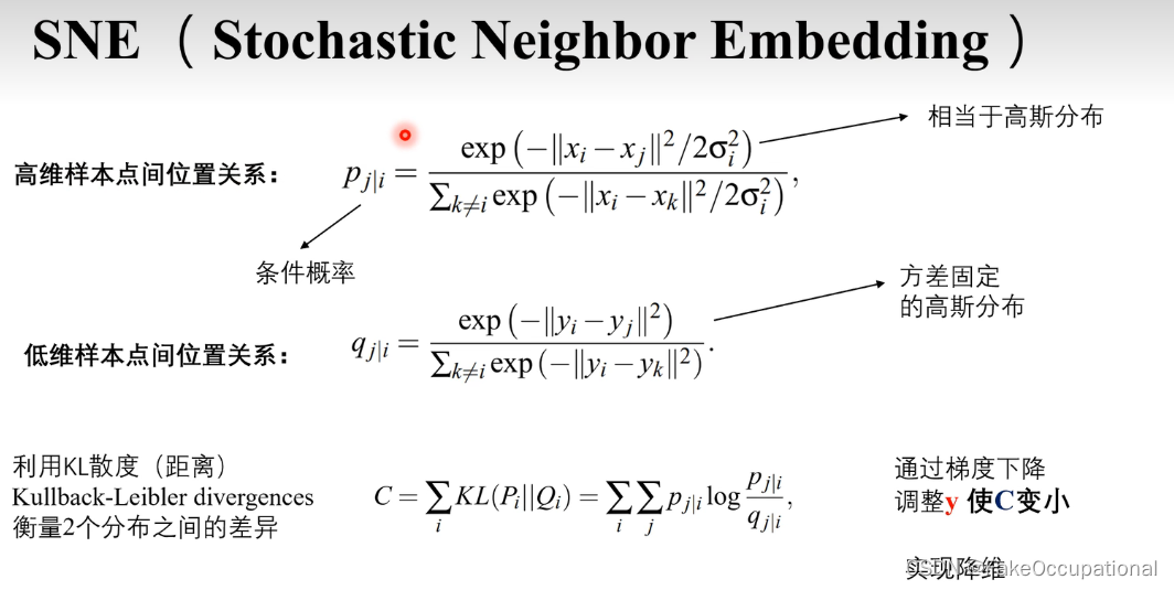
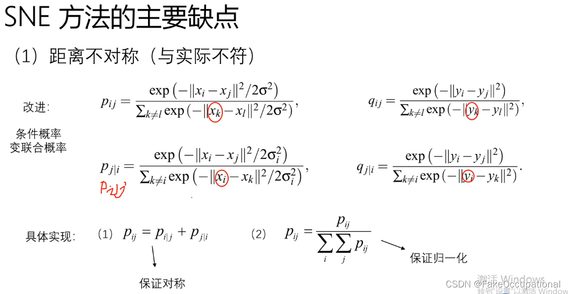
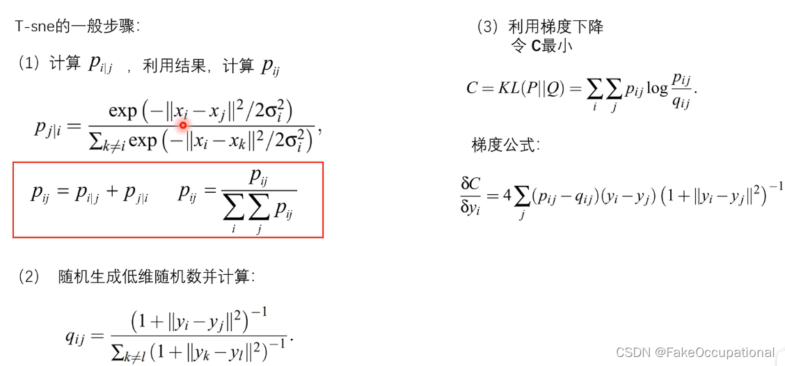
t-sne 数据可视化的数学解释

参考与更多
pytorch官方保存加载模型教程(包含使用以 TorchScript 格式导出/加载模型)
模型字典的修改: https://discuss.pytorch.org/t/how-to-load-part-of-pre-trained-model/1113/2
scikit-learn.org
https://github.com/shivanichander/tSNE/blob/master/Code/tSNE%20Code.ipynb
t-SNE:最好的降维方法之一 - 知乎 (zhihu.com)
https://discuss.pytorch.org/t/changing-state-dict-value-is-not-changing-model/88695/2
model = nn.Linear(1, 1)
print(model.weight)
# ISOMAP https://scikit-learn.org.cn/view/452.html
from sklearn.manifold import Isomap
digits_final = Isomap(n_components=2).fit_transform(res)
边栏推荐
猜你喜欢

Efficient use of RecyclerView Section 1
OPPO在FaaS领域的探索与思考

leetcode303 Weekly Match Replay

TextBlock控件入门基础工具使用用法,取上法入门

What is the difference between BI software in the domestic market?
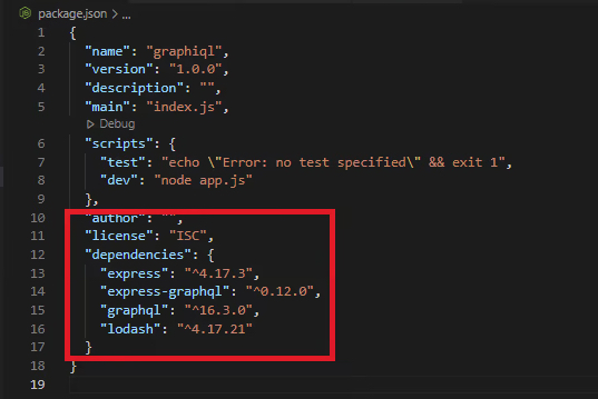
Visualize GraphQL schemas with GraphiQL
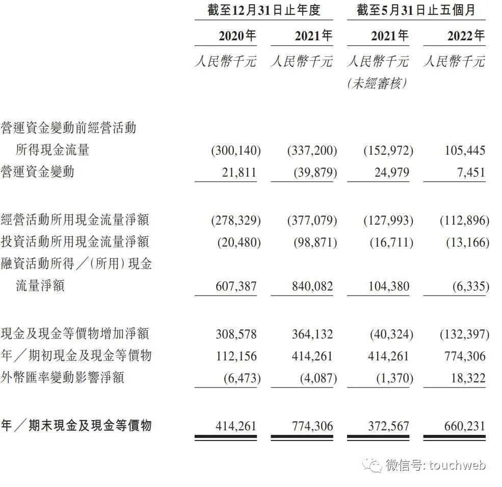
思路迪医药冲刺港股:5个月亏2.9亿 泰格医药与先声药业是股东
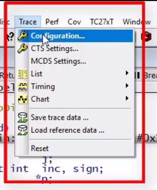
TRACE32 - SNOOPer-based variable logging

安装Xshell并使用其进行Ymodem协议的串口传输
RecyclerView的高效使用第一节
随机推荐
R language test whether the sample conforms to normality (test whether the sample comes from a normally distributed population): shapiro.test function tests whether the sample conforms to the normal d
Implementing click on the 3D model in RenderTexture in Unity
Synchronized and volatile interview brief summary
763.划分字母区间——之打开新世界
border控件的使用
R语言ggplot2可视化:使用ggpubr包的ggmaplot函数可视化MA图(MA-plot)、font.legend参数和font.main参数设置标题和图例字体加粗
基于ABP实现DDD
Ubantu专题4:xshell、xftp连接接虚拟机以及设置xshell复制粘贴快捷键
【CUDA学习笔记】初识CUDA
What is the difference between BI software in the domestic market?
DBeaver连接MySQL 8.x时Public Key Retrieval is not allowed 错误解决
Efficient use of RecyclerView Section 1
WeChat chat record search in a red envelope
Kubernetes常用命令
R语言计算时间序列数据的移动平均值(滚动平均值、例如5日均线、10日均线等):使用zoo包中的rollmean函数计算k个周期移动平均值
贪吃蛇项目(简单)
TRACE32 - Common Operations
华医网冲刺港股:5个月亏2976万 红杉与姚文彬是股东
名创优品斥资6.95亿购买创始人叶国富所持办公楼股权
json到底是什么(c# json)