当前位置:网站首页>Deep Blue Academy - Fourteen Lectures of Visual SLAM - Chapter 4 Homework
Deep Blue Academy - Fourteen Lectures of Visual SLAM - Chapter 4 Homework
2022-08-02 05:23:00 【hello689】
Fourth class homework
2.图像去畸变
The main content of this question is to achieve image de-distortion according to the provided formulas and parameters.
Coordinate change formula before and after distortion:
{ x d i s t o r t e d = x ( 1 + k 1 r 2 + k 2 r 4 ) + 2 p 1 x y + p 2 ( r 2 + 2 x 2 ) y d i s t o r t e d = y ( 1 + k 1 r 2 + k 2 r 4 ) + p 1 ( r 2 + 2 y 2 ) + 2 p 2 x y \begin{cases} x_{distorted} = x(1+k_1r^2+k_2r^4)+2p_1xy+p_2(r^2+2x^2) \\ y_{distorted} = y(1+k_1r^2+k_2r^4)+p_1(r^2+2y^2)+2p_2xy \end{cases} { xdistorted=x(1+k1r2+k2r4)+2p1xy+p2(r2+2x2)ydistorted=y(1+k1r2+k2r4)+p1(r2+2y2)+2p2xy
where the given parameters are :
k 1 = − 0.28340811 , k 2 = 0.07395907 , p 1 = 0.00019359 , p 2 = 1.76187114 e − 05 相 机 内 参 : f x = 458.654 , f y = 457.296 , c x = 367.215 , c y = 248.375 k_1 = -0.28340811,k_2 = 0.07395907,p_1 = 0.00019359,p_2=1.76187114e-05 \\ 相机内参:\\ f_x = 458.654,f_y=457.296,c_x=367.215,c_y=248.375 k1=−0.28340811,k2=0.07395907,p1=0.00019359,p2=1.76187114e−05相机内参:fx=458.654,fy=457.296,cx=367.215,cy=248.375
Dewarping the core part of the code:
 // start your code here
//计算归一化坐标
double x = (u - cx)/fx;
double y = (v - cy)/fy;
double r = sqrt(x*x + y*y);
//Calculate radial and tangentially distorted coordinates
double x_distorted = x * (1 + k1 * r * r + k2 * r * r * r * r) + 2 * p1 * x * y + p2 * (r * r + 2 * x * x);
double y_distorted = y * (1 + k1 * r * r + k2 * r * r * r * r) + p1 * (r * r + 2 * y * y) + 2 * p2 * x * y;
//计算像素
u_distorted = fx * x_distorted + cx;
v_distorted = fy * y_distorted + cy;
// end your code here
De-distortion rendering:

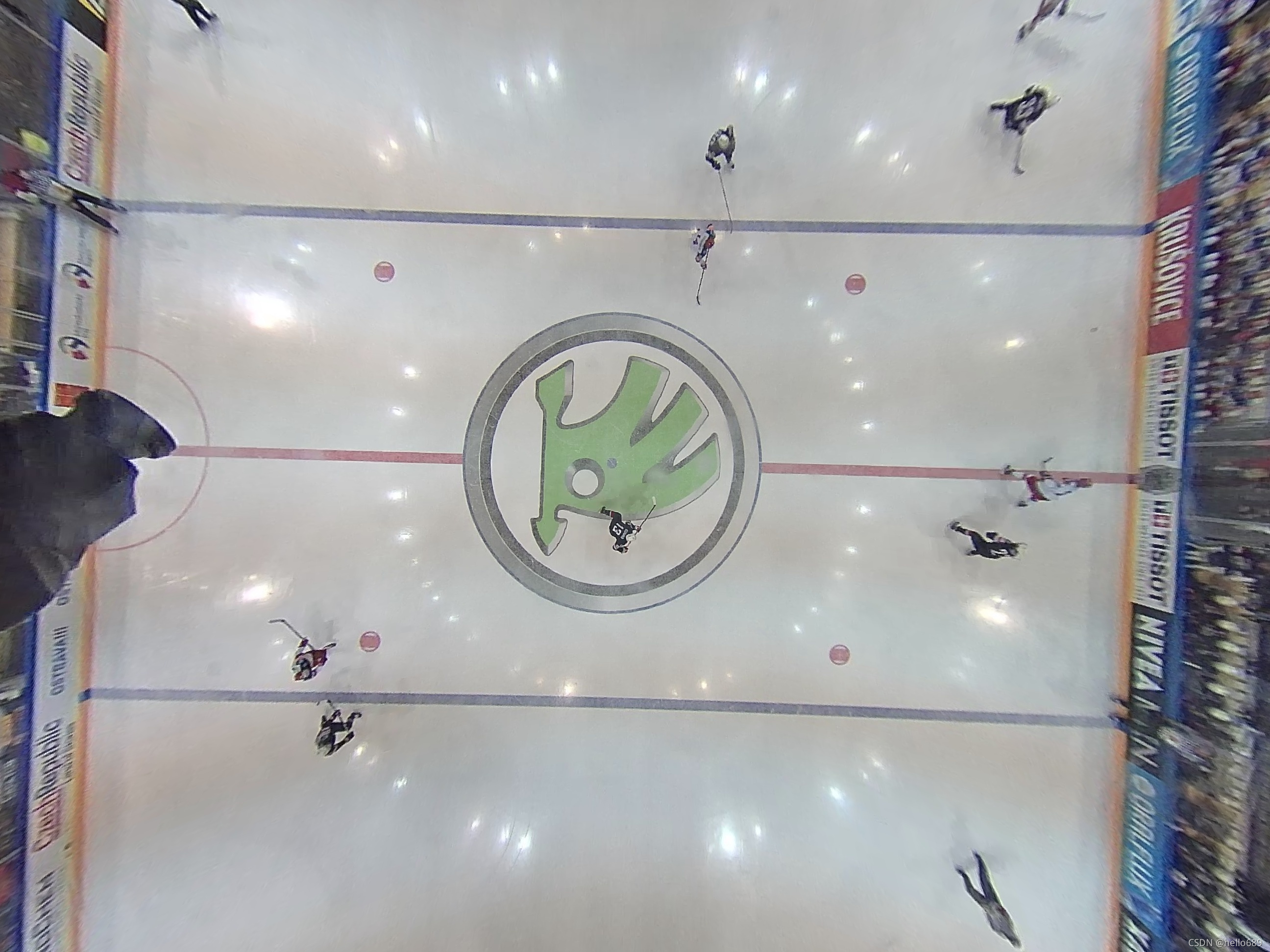
3.鱼眼模型与去畸变
请说明鱼眼相机相比于普通针孔相机在SLAM 方面的优势.
One of the most important advantages of fisheye cameras is that they have a wider field of view than ordinary pinhole cameras.So you can be sure for a while,Bring as many visual features as possible into the camera's field of view,Thereby improving the perception of the surrounding environment.
请整理并描述OpenCV 中使用的Fisheye Distortion模型(等距投影)是如何定义的,它与上题的畸变模型
有何不同.参考资料:
- OpenCV: Fisheye camera model
- https://blog.csdn.net/KYJL888/article/details/117423950
- https://blog.csdn.net/weixin_43304707/article/details/113261307
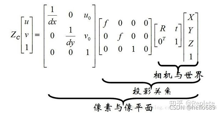
模型定义(也叫kannala-brandt模型,There are various fisheye distortion models):
Set a point in the world coordinate systemP,The coordinates of the point are used in a matrixX表示.Vector coordinates in the camera coordinate systemP为:
X c = R X + T Xc = RX + T Xc=RX+T
其中,R是旋转矩阵,旋转向量omAfter Rodrigues transformation.XcThe three quantities are respectivelyx,y,z;
x = X c 1 y = Y c 2 z = X c 3 x = Xc_1 \\ y = Yc_2\\ z = Xc_3 x=Xc1y=Yc2z=Xc3
PThe pinhole projection coordinates of [a,b]:
a = x / z a n d b = y / z r 2 = a 2 + b 2 θ = arctan ( r ) a=x/z \space and \space b = y/z\\ r^2=a^2+b^2\\ \theta = \arctan(r) a=x/z and b=y/zr2=a2+b2θ=arctan(r)
注:在OpenCV的文档中,如下图所示, θ = a t a n ( r ) \theta = atan(r) θ=atan(r),represents the arc tangent,也可以描述成 θ = arctan ( r ) \theta = \arctan(r) θ=arctan(r).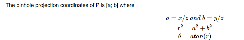
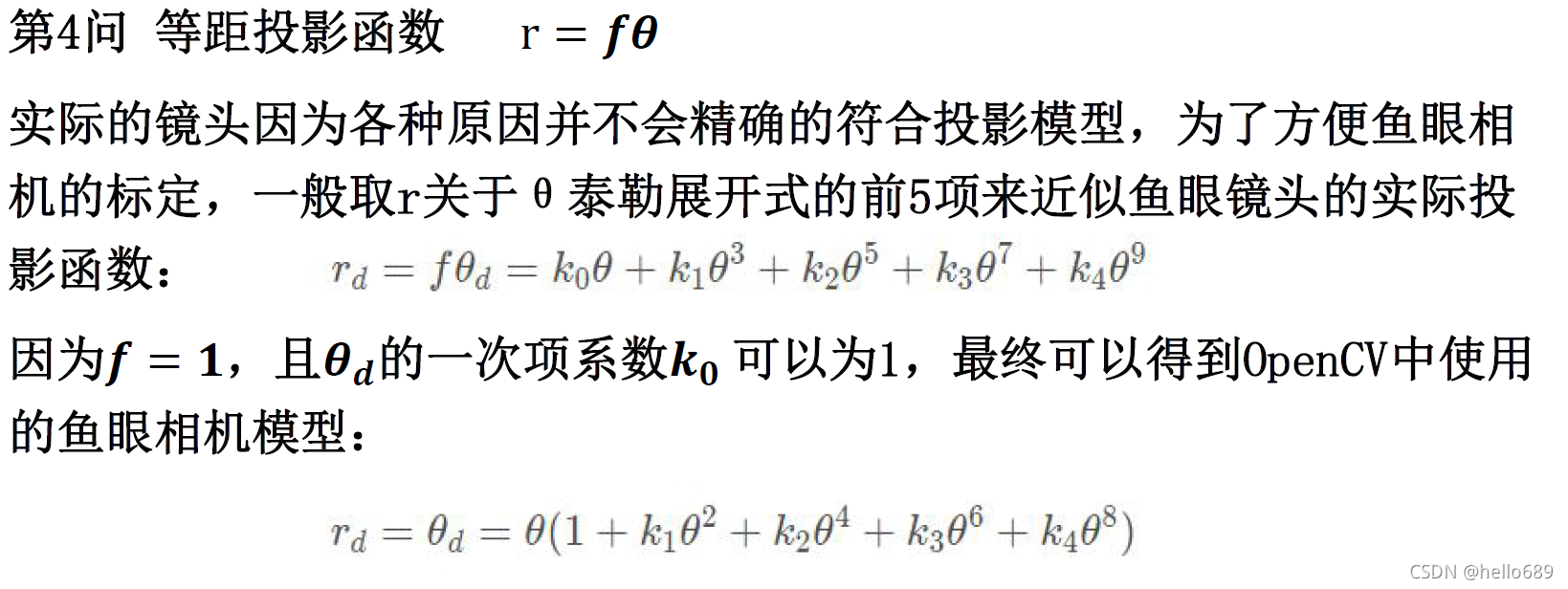
Fisheye Distortion:
θ d = θ ( 1 + k 1 θ 2 + k 2 θ 3 + k 3 θ 6 + k 4 θ 8 ) \theta_d = \theta(1+k_1\theta^2+k_2\theta^3+k_3\theta^6+k_4\theta^8) θd=θ(1+k1θ2+k2θ3+k3θ6+k4θ8)
The coordinates of the distorted point are [ x ′ ; y ′ ] [x^{'};y^{'}] [x′;y′]:
x ′ = ( θ d / r ) a y ′ = ( θ d / r ) b x^{'} = (\theta_d/r)a\\ y^{'} = (\theta_d/r)b x′=(θd/r)ay′=(θd/r)b
最后,Convert to pixel coordinate system,The final pixel coordinate vector is [u;v], α \alpha α为偏度系数:
u = f x ( x ′ + α y ′ ) + c x v = f y y ′ + c y u = f_x(x^{'}+\alpha y^{'})+c_x\\ v = f_y y^{'}+c_y u=fx(x′+αy′)+cxv=fyy′+cy
The difference from the distortion model in the previous question:The distortion model of the above question includes radial and tangential distortions.The fisheye camera of this question is only given θ d \theta_d θdA type of distortion.我注意到,Solving for the final pixel coordinates u u u时,Added one to the fisheye camera conversion α y ′ \alpha y^{'} αy′与y有关的变量,Different from the previous model.完成fisheye.cpp 文件中的内容.针对给定的图像,实现它的畸变校正.要求:通过手写方式实现,
不允许调用OpenCV 的API.通过上述公式,The core code to implement dewarping is shown below:
 double a = (u-cx)/fx, b = (v-cy)/fy;
double r = sqrt(a*a + b*b);
double theta = atan(r);
double theta_2 = theta*theta;
double theta_4 = theta_2*theta_2;
double theta_6 = theta_4*theta_2;
double theta_8 = theta_4*theta_4;
double theta_d = theta*(1+k1*theta_2+k2*theta_4+k3*theta_6+k4*theta_8);

double x_distorted = (theta_d / r)*a;
double y_distorted = (theta_d / r)*b;

u_distorted = fx*(x_distorted + 0.01*y_distorted)+cx;
v_distorted = fy*y_distorted + cy;
The effect of removing fisheye distortion:
Why in this image,我们令畸变参数k1, . . . , k4 = 0,依然可以产生去畸变的效果?
θ d = θ ( 1 + k 1 θ 2 + k 2 θ 3 + k 3 θ 6 + k 4 θ 8 ) \theta_d = \theta(1+k_1\theta^2+k_2\theta^3+k_3\theta^6+k_4\theta^8) θd=θ(1+k1θ2+k2θ3+k3θ6+k4θ8)The fisheye camera finally reaches the imaging unit through the refraction of multiple lenses.Kannala-BrandtFisheye Distortion模型,It's actually about the angle of incidence θ \theta θ 的奇函数,因此鱼眼镜头的畸变也是对 θ \theta θ 的畸变,It cannot be described by simple radial and tangential distortion polynomials.而 k 1 , ⋯ , k 4 k_1,\cdots ,k_4 k1,⋯,k4,is the radial distortion coefficient determined by camera calibration,这里可以暂时忽略.因此令 k 1 , ⋯ , k 4 k_1,\cdots ,k_4 k1,⋯,k4为0,The effect of removing the distortion can still be clearly displayed.
正确答案:Take the first five terms of Taylor expansion to approximate the fisheye model,k1-k4取0,Equivalent to only approximating the first term,So the de-distortion operation can still be done.
在鱼眼模型中,去畸变是否带来了图像内容的损失?如何避免这种图像内容上的损失呢?
Fisheye diagrams are generally circular,The information at the edge is compressed very densely,After removing the distortion, the middle part of the original image will be well preserved,The edge position is generally stretched very seriously、视觉效果差,So excision is usually done,Therefore, there will definitely be a loss of image content.Increases the size of the image when dewarped,Or use monocular and fisheye camera images for fusion,Complete missing information.
4.双目视差的使用
理论部分
推导双目相机模型下,视差与 X Y Z XYZ XYZ坐标的关系式.请给出由像素坐标加视差 u , v , d u, v, d u,v,d推导 X Y Z XYZ XYZ
与已知 X Y Z XYZ XYZ推导 u , v , d u, v, d u,v,d两个关系.First give the world coordinate system、相机坐标系、图像坐标系、像素坐标系的关系:
img source:https://zhuanlan.zhihu.com/p/421453976
set a pointP在成像平面上的两个点 P L 、 P R P_L、P_R PL、PR的坐标分别是 ( x l , y l ) ( x r , y r ) (x^l,y^l)(x^r,y^r) (xl,yl)(xr,yr):
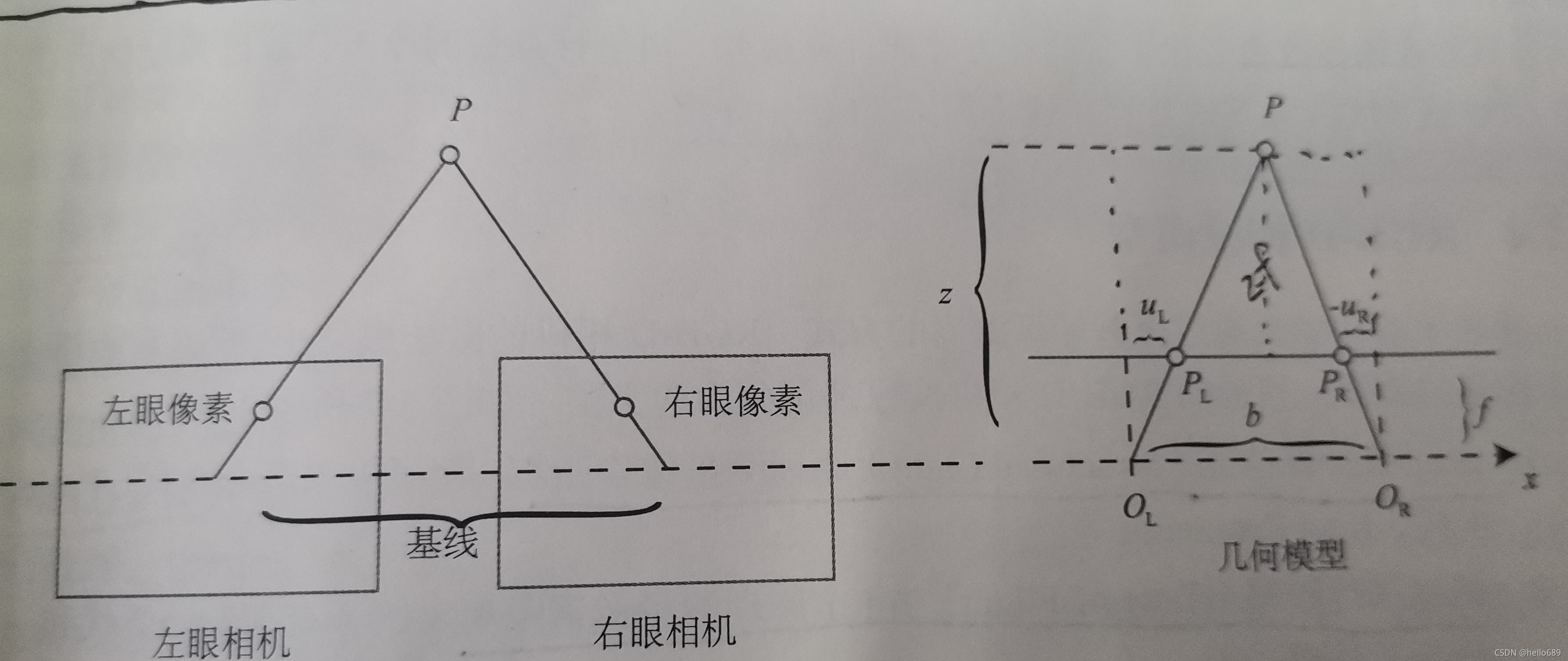
根据三角形 △ P P L P R \bigtriangleup PP_LP_R △PPLPR和 △ P O L O R \bigtriangleup PO_LO_R △POLORThere are similar relationships:
z − f z = b − u L + u R b \frac{z-f}{z} = \frac{b-u_L+u_R}{b} zz−f=bb−uL+uR
整理可得:
z = f b d , d = x l − x r z = \frac{fb}{d},d=x_l-x_r z=dfb,d=xl−xr
其中d定义为左右图的横坐标之差,称为视差.f为相机的焦距,bis the distance between the two cameras,也就是基线.得到深度值 z z z后,即可得出目标点的三维坐标:
{ u = b x l d v = b y 1 d z = f b d \begin{cases} u = \frac{bx_l}{d}\\ v = \frac{by_1}{d}\\ z = \frac{fb}{d} \end{cases} ⎩⎪⎨⎪⎧u=dbxlv=dby1z=dfb推导在右目相机下该模型将发生什么改变.
In the parallax piece,Use the right eye camera coordinates to subtract the left eye camera coordinates,d = x_r - x_l.Use the projection point of the right eye camera,Also use the extrinsic parameters of the left eye camera.
编程部分
核心部分代码:
// start your code here (~6 lines)
// 根据双目模型计算 point 的位置
double x = (u - cx) / fx;
double y = (v - cy) / fy;
double depth = fx * d / (disparity.at<char>(v, u));
point[0] = x * depth;
point[1] = y * depth;
point[2] = depth;

pointcloud.push_back(point);
// end your code here
运行效果:

5.矩阵运算微分
设变量为 x ∈ R N x \in \mathbb{R}^N x∈RN,那么:
矩阵 A ∈ R N × N A \in \mathbb{R}^{N \times N} A∈RN×N,那么d(Ax)/dx 是什么?
d ( A X ) d x = A T \frac{d(AX)}{dx}= A^T dxd(AX)=AT矩阵 A ∈ R N × N A \in \mathbb{R}^{N \times N} A∈RN×N,那么 d ( x T A x ) / d x d(x^TAx)/dx d(xTAx)/dx是什么?
d ( x T A x ) d x = ( d x ) T A x + x T A d x d x = d x T A x + d x T A T x d x = ( A + A T ) x \frac{d(x^TAx)}{dx} = \frac{(dx)^TAx+x^TAdx}{dx}= \frac{dx^TAx+dx^TA^Tx}{dx} = (A+A^T)x dxd(xTAx)=dx(dx)TAx+xTAdx=dxdxTAx+dxTATx=(A+AT)x证明:
x T A x = t r ( A x x T ) 证 明 : 左 式 = x T A x = [ x 1 , x 2 , ⋯ , x n ] ⋅ [ a 11 , a 12 , ⋯ , a 1 n a 21 , a 22 , ⋯ , a 2 n ⋯ a n 1 , a n 2 , ⋯ , a n n ] ⋅ [ x 1 x 2 ⋯ x n ] = x 1 ∑ i = 1 n a 1 i x i + x 2 ∑ i = 1 n a 2 i x i + ⋯ + x n ∑ i = 1 n a n i x i 右 式 = t r ( A x x T ) = t r ( [ a 11 , a 12 , ⋯ , a 1 n a 21 , a 22 , ⋯ , a 2 n ⋯ a n 1 , a n 2 , ⋯ , a n n ] ⋅ [ x 1 x 2 ⋯ x n ] ⋅ [ x 1 , x 2 , ⋯ , x n ] ) = t r ( [ a 11 , a 12 , ⋯ , a 1 n a 21 , a 22 , ⋯ , a 2 n ⋯ a n 1 , a n 2 , ⋯ , a n n ] ⋅ [ x 1 x 1 , x 1 x 2 , ⋯ , x 1 x n x 2 x 1 , a 2 x 2 , ⋯ , x 2 x n ⋯ x n x 1 , x n x 2 , ⋯ , x n x n ] ) = x 1 ∑ i = 1 n a 1 i x i + x 2 ∑ i = 1 n a 2 i x i + ⋯ + x n ∑ i = 1 n a n i x i 得 证 x^T Ax = tr(Axx^T)\\ 证明:\\ \begin{aligned} 左式 &= x^TAx\\ &= \begin{bmatrix} x_1,x_2,\cdots,x_n \end{bmatrix} \cdot \begin{bmatrix} a_{11},a_{12},\cdots,a_{1n}\\ a_{21},a_{22},\cdots,a_{2n}\\ \cdots\\ a_{n1},a_{n2},\cdots,a_{nn}\\ \end{bmatrix}\cdot \begin{bmatrix} x_1\\x_2\\ \cdots\\x_n \end{bmatrix} \\&= x_1\sum_{i=1 }^{n}a_{1i}x_i+x_2\sum_{i=1 }^{n}a_{2i}x_i+\cdots+x_n\sum_{i=1 }^{n}a_{ni}x_i\\ 右式 &=tr(Axx^T) \\&= tr\begin{pmatrix} \begin{bmatrix} a_{11},a_{12},\cdots,a_{1n}\\ a_{21},a_{22},\cdots,a_{2n}\\ \cdots\\ a_{n1},a_{n2},\cdots,a_{nn}\\ \end{bmatrix}\cdot \begin{bmatrix} x_1\\x_2\\ \cdots\\x_n \end{bmatrix} \cdot \begin{bmatrix} x_1,x_2,\cdots,x_n \end{bmatrix} \end{pmatrix}\\&= tr\begin{pmatrix} \begin{bmatrix} a_{11},a_{12},\cdots,a_{1n}\\ a_{21},a_{22},\cdots,a_{2n}\\ \cdots\\ a_{n1},a_{n2},\cdots,a_{nn}\\ \end{bmatrix}\cdot \begin{bmatrix} x_1x_1,x_1x_2,\cdots,x_1x_n\\ x_2x_1,a_2x_2,\cdots,x_2x_n\\ \cdots\\ x_nx_1,x_nx_2,\cdots,x_nx_n\\ \end{bmatrix} \end{pmatrix}\\&= x_1\sum_{i=1 }^{n}a_{1i}x_i+x_2\sum_{i=1 }^{n}a_{2i}x_i+\cdots+x_n\sum_{i=1 }^{n}a_{ni}x_i\\ \end{aligned}\\ 得证 xTAx=tr(AxxT)证明:左式右式=xTAx=[x1,x2,⋯,xn]⋅⎣⎢⎢⎡a11,a12,⋯,a1na21,a22,⋯,a2n⋯an1,an2,⋯,ann⎦⎥⎥⎤⋅⎣⎢⎢⎡x1x2⋯xn⎦⎥⎥⎤=x1i=1∑na1ixi+x2i=1∑na2ixi+⋯+xni=1∑nanixi=tr(AxxT)=tr⎝⎜⎜⎛⎣⎢⎢⎡a11,a12,⋯,a1na21,a22,⋯,a2n⋯an1,an2,⋯,ann⎦⎥⎥⎤⋅⎣⎢⎢⎡x1x2⋯xn⎦⎥⎥⎤⋅[x1,x2,⋯,xn]⎠⎟⎟⎞=tr⎝⎜⎜⎛⎣⎢⎢⎡a11,a12,⋯,a1na21,a22,⋯,a2n⋯an1,an2,⋯,ann⎦⎥⎥⎤⋅⎣⎢⎢⎡x1x1,x1x2,⋯,x1xnx2x1,a2x2,⋯,x2xn⋯xnx1,xnx2,⋯,xnxn⎦⎥⎥⎤⎠⎟⎟⎞=x1i=1∑na1ixi+x2i=1∑na2ixi+⋯+xni=1∑nanixi得证
6.高斯牛顿法的曲线拟合实验
定义误差为:
e i = y i − exp ( a x i 2 + b x i + c ) e_i = y_i-\exp(ax_i^2+bx_i+c) ei=yi−exp(axi2+bxi+c)
每个误差项对于状态变量的导数:
∂ e i ∂ a = − x i 2 exp ( a x i 2 + b x i + c ) ∂ e i ∂ b = − x i exp ( a x i 2 + b x i + c ) ∂ e i ∂ c = − exp ( a x i 2 + b x i + c ) \frac{\partial e_i}{\partial a} = -x_i^2\exp(ax_i^2+bx_i+c)\\ \frac{\partial e_i}{\partial b} = -x_i\exp(ax_i^2+bx_i+c)\\ \frac{\partial e_i}{\partial c} = -\exp(ax_i^2+bx_i+c)\\ ∂a∂ei=−xi2exp(axi2+bxi+c)∂b∂ei=−xiexp(axi2+bxi+c)∂c∂ei=−exp(axi2+bxi+c)
根据该公式,Data fitting was performed using the Gauss-Newton method,主要部分代码如下:
// start your code here
double error = 0;   // 第i个数据点的计算误差
error = yi - exp(ae * xi * xi + be*xi + ce); // 填写计算error的表达式
Vector3d J; // 雅可比矩阵
J[0] = -xi*xi*exp(ae * xi * xi + be*xi + ce);  // de/da
J[1] = -xi* exp(ae * xi * xi + be*xi + ce);  // de/db
J[2] = -exp(ae * xi * xi + be*xi + ce);  // de/dc

H += J * J.transpose(); // GN近似的H
b += -error * J;
// end your code here

// 求解线性方程 Hx=b,建议用ldlt
// start your code here
Vector3d dx = H.ldlt().solve(b);
// end your code here
运行结果:

7.批量最大似然估计
1.可以定义矩阵 H H H,使得批量误差为 e = z − H x e = z − Hx e=z−Hx.请给出此处 H H H的具体形式.
e = z − H x x = [ x 0 , x 1 , x 2 , x 3 ] T z = [ v 1 , v 2 , v 3 , y 1 , y 2 , y 3 ] T e = z-Hx\\ x = [x_0,x_1,x_2,x_3]^T\\ z=[v_1,v_2,v_3,y_1,y_2,y_3]^T e=z−Hxx=[x0,x1,x2,x3]Tz=[v1,v2,v3,y1,y2,y3]T
所以H的大小应该是 6 × 4 6\times4 6×4,且需要满足:
x k = x k − 1 + v k + w k y k = x k + n k x_k = x_{k-1}+v_k+w_k\\ y_k = x_k+n_k xk=xk−1+vk+wkyk=xk+nk
e = z − H x = [ v 1 v 2 v 3 y 1 y 2 y 3 ] − H ⋅ [ x 0 x 1 x 2 x 3 ] = [ v 1 − ( x 1 − x 0 ) v 2 − ( x 2 − x 1 ) v 3 − ( x 3 − x 2 ) y 1 − x 1 y 2 − x 2 y 3 − x 3 ] \begin{aligned} e &= z-Hx\\&= \begin{bmatrix} v_1\\v_2\\v_3\\y_1\\y_2\\y_3 \end{bmatrix}-H\cdot \begin{bmatrix} x_0\\x_1\\x_2\\x_3 \end{bmatrix}\\&= \begin{bmatrix} v_1-(x_1-x_0)\\ v_2-(x_2-x_1) \\ v_3-(x_3-x_2)\\ y_1-x_1\\ y_2-x_2\\ y_3-x_3 \end{bmatrix}\\ \end{aligned} e=z−Hx=⎣⎢⎢⎢⎢⎢⎢⎡v1v2v3y1y2y3⎦⎥⎥⎥⎥⎥⎥⎤−H⋅⎣⎢⎢⎡x0x1x2x3⎦⎥⎥⎤=⎣⎢⎢⎢⎢⎢⎢⎡v1−(x1−x0)v2−(x2−x1)v3−(x3−x2)y1−x1y2−x2y3−x3⎦⎥⎥⎥⎥⎥⎥⎤
所以H为:
H = [ − 1 1 0 0 0 − 1 1 0 0 0 − 1 1 0 1 0 0 0 0 1 0 0 0 0 1 ] H = \begin{bmatrix} -1&1&0&0\\ 0&-1&1&0\\ 0&0&-1&1\\ 0&1&0&0\\ 0&0&1&0\\ 0&0&0&1 \end{bmatrix} H=⎣⎢⎢⎢⎢⎢⎢⎡−1000001−1010001−1010001001⎦⎥⎥⎥⎥⎥⎥⎤
参考博客:https://blog.csdn.net/floatinglong/article/details/116202102
- W − 1 W^{-1} W−1为此问题的信息矩阵,即高斯分布协方差矩阵之逆.
Σ = d i a g ( Q 1 , Q 2 , Q 3 , R 1 , R 2 , R 3 ) \Sigma = diag (Q_1,Q_2,Q_3,R_1,R_2,R_3) Σ=diag(Q1,Q2,Q3,R1,R2,R3)
存在唯一解
目标函数简化为:
x M L E ∗ = a r g m a x ( e T Σ − 1 e ) x^*_{MLE} = argmax(e^T\Sigma^{-1}e)\\ xMLE∗=argmax(eTΣ−1e)
唯一解:
x M L E ∗ = ( H T Σ − 1 H ) − 1 H T Σ − 1 y x^*_{MLE} = (H^T\Sigma^{-1}H)^{-1}H^T\Sigma^{-1}y xMLE∗=(HTΣ−1H)−1HTΣ−1y
github地址: https://github.com/ximing1998/slam-learning.git
国内gitee地址:https://gitee.com/ximing689/slam-learning.git
边栏推荐
猜你喜欢

科研笔记(八) 深度学习及其在 WiFi 人体感知中的应用(上)

flasgger手写phpwind接口文档
吴恩达机器学习系列课程笔记——第十八章:应用实例:图片文字识别(Application Example: Photo OCR)

shell脚本的基础知识
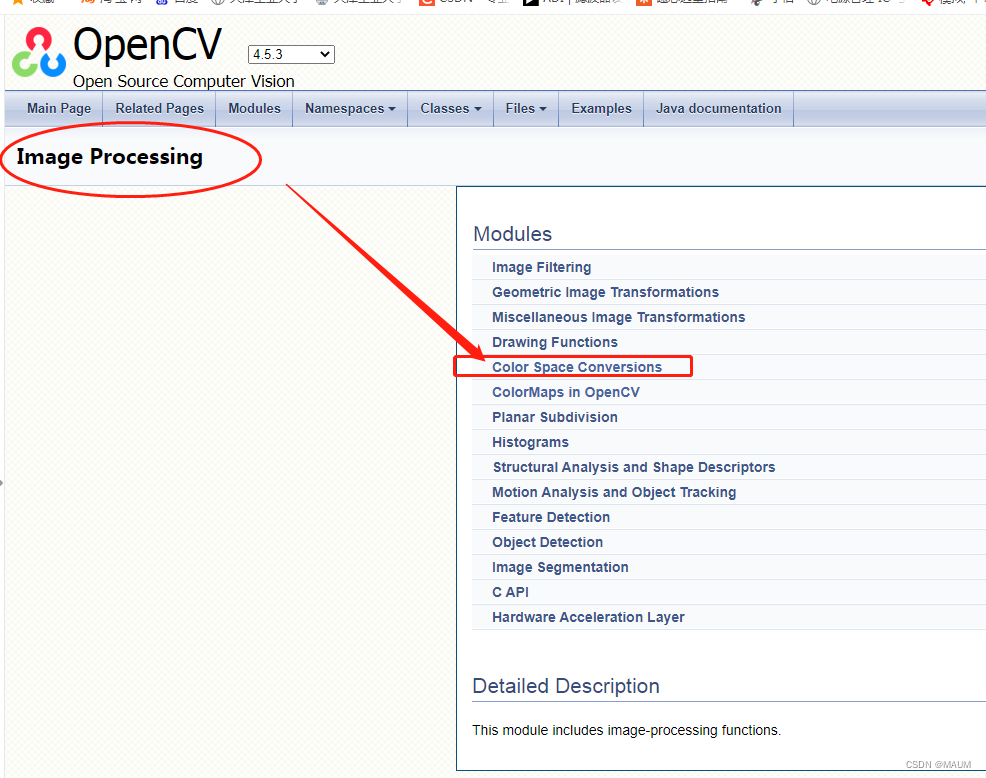
QT中更换OPENCV版本(3->4),以及一些宏定义的改变

SLSA 框架与软件供应链安全防护

如何将 DevSecOps 引入企业?
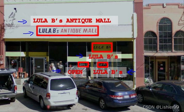
Andrew Ng's Machine Learning Series Course Notes - Chapter 18: Application Example: Image Text Recognition (Application Example: Photo OCR)
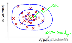
吴恩达机器学习系列课程笔记——第十五章:异常检测(Anomaly Detection)

Win8.1下QT4.8集成开发环境的搭建
随机推荐
单目3D目标检测之入门
JS事件循环机制
位居榜首 | 未来智安荣登CCIA「2022年中国网安产业潜力之星」榜单
音视频文件的码率与大小计算
Gartner 权威预测未来4年网络安全的8大发展趋势
matlab作图显示中文正常,保存图片中文乱码
Class ‘PHPWord_Writer_Word2003‘ not found
吴恩达机器学习系列课程笔记——第十三章:聚类(Clustering)
The slave I/O thread stops because master and slave have equal MySQL server ids
强化学习(西瓜书第16章)思维导图
el-dropdown(下拉菜单)的入门学习
剩余参数、数组对象的方法和字符串扩展的方法
心余力绌:企业面临的软件供应链安全困境
深蓝学院-视觉SLAM十四讲-第六章作业
单目三维目标检测之CaDDN论文阅读
GO Module的依赖管理(二)
SCI期刊最权威的信息查询步骤!
2022 开源软件安全状况报告:超 41% 的企业对开源安全没有足够的信心
ScholarOne Manuscripts提交期刊LaTeX文件,无法成功转换PDF!
Nexus 5手机使用Nexmon工具获取CSI信息