[deep learning] activation function (sigmoid, etc.), forward propagation, back propagation and gradient optimization; optimizer. zero_ grad(), loss. backward(), optimizer. Function and principle of st

use Matt Mazur Example , Let's simply tell the reader the derivation process （ It's actually a chain ）！

First initialize the weight and offset , The results are as follows ：

One 、 Activation function

1.1 What is an activation function ？

Activation functions can be divided into Linear activation function （ Linear equations control input to output mapping , Such as f(x)=x etc. ） And the nonlinear activation function （ Nonlinear equations control input-output mapping , such as Sigmoid、Tanh、ReLU、LReLU、PReLU、Swish etc. ）

Activation function is to introduce nonlinear factors into neural network , Various curves can be fitted by activating function neural network . Activation function can be divided into saturation activation function （Saturated Neurons） And unsaturated functions （One-sided Saturations）.Sigmoid and Tanh Is the saturation activation function , and ReLU And its variant is unsaturated activation function . Unsaturated activation function has the following advantages ：

1. The unsaturated activation function can solve the gradient vanishing problem .
2. The unsaturated activation function can accelerate the convergence .

1.2 Common activation functions

1.2.1 Sigmoid function

$SigmoidLetterCountalsoIt\text{'}s\; calledLogisticLetterCount$, For hidden layer neuron output , The value range is (0,1), It maps a real number to (0,1) The range of , It can be used for secondary classification . The effect is better when the feature difference is more complex or the difference is not particularly large .sigmoid Is a very common activation function , The expression of the function is as follows ：

The image is similar to a S Shape curve ：

• Sigmoid The output range of the function is 0 To 1. Because the output value is limited to 0 To 1, So it normalizes the output of each neuron ;
• Functions are differentiable . This means that any two points can be found sigmoid The slope of the curve ;
• however Sigmoid Function approach 0 and 1 The rate of change will flatten out , in other words ,Sigmoid The gradient of is close to 0. Neural networks use Sigmoid When the function is activated for back propagation , Output close to 0 or 1 The gradient of the neurons is close to 0. These neurons are called saturated neurons . therefore , The weights of these neurons don't update . Besides , The weights of the neurons connected to these neurons are also updated very slowly . The problem is called $ladderdegreeeliminateloss$.

1.2.2 ReLU Activation function

ReLU Function is also called modified linear element （Rectified Linear Unit）, It's a piecewise linear function , It makes up for sigmoid Function and tanh Gradient vanishing problem of function , It is widely used in the current deep neural network .ReLU A function is essentially a ramp （ramp） function , The formula and function image are as follows ：

Images ：

• When the input is positive , Derivative is 1, The gradient vanishing problem is improved to some extent , Accelerate the convergence rate of gradient descent ;
• It's much faster .ReLU There is only a linear relationship in the function , So it's faster than sigmoid and tanh faster .
  Considered biologically reasonable （Biological Plausibility）, For example, unilateral inhibition 、 Wide boundaries of excitement （ That is, the level of excitement can be very high ）

1.2.3 Softmax Activation function

Softmax Is an activation function for multi class classification problems , In the multi class classification problem , More than two class tags require class membership . For length is K Any real vector of ,Softmax It can be compressed to a length of K, Values in （0,1） Within the scope of , And the sum of the elements in the vector is 1 The real vector of . The function expression is as follows ：

Images ：

Function example ：$OnelikeuseCome\; ondischargestaynetworkCollateralmostaftertransportOutvariousclassotherGeneralratevalue$

Softmax Deficiency of activation function ：

• It's nondifferentiable at zero ;
• The gradient of negative input is zero , This means that for the activation of the region , Weights are not updated during back propagation , So it produces dead neurons that never activate .

1.2.4 Reference to other activation functions Deep learning notes ： How to understand activation function ？（ Common activation functions attached ）

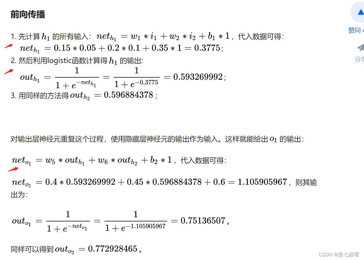
Two 、 Forward propagation reasoning inference Calculation example

• Calculation neth1=w*i+b
• Calculate by activation function outh1
• Calculate the next level neth2、 Through the activation function of the next layer
• Calculation error Etotal

3、 ... and 、 Back propagation backward Calculation example

• The chain rule ： Calculation Etotal About w5 Partial derivative of , Actually = Calculation Etotal About outh1 Partial derivative of * outh1 About neth1 Partial derivative of * neth1 About w5 Partial derivative of
• Corresponding to three functions respectively ： error function 、 Activation function 、y=w*i+b

With the same steps, you can update all w：

Reference resources ：

• Deep learning — Specific cases of back propagation
• Matt Mazur
• 【 Deep learning theory 】 Pure formula hand push + Code —— Back propagation of neural networks + gradient descent

Four 、 Gradient optimization

4.1 How to minimize an arbitrary function ？

Look closely at the cost function , In the form of Y=X². In Cartesian coordinates , This is a parabolic equation , It is graphically represented as follows ：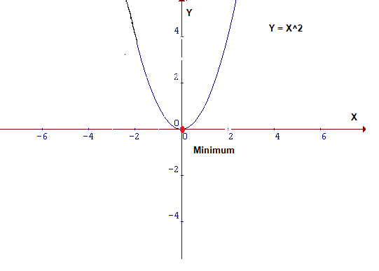

To minimize the above function , Need to find one x, The function can produce a small value at this point Y, That is, the red dot in the figure .

Because this is a two-dimensional image , Therefore, it is easy to find its minimum value , But in $dimensiondegreeThanaBig$ Under the circumstances , It will be more complicated . In this case , An algorithm needs to be designed to locate the minimum , This algorithm is called gradient descent algorithm (Gradient Descent).

Gradient descent is one of the most popular algorithms for model optimization , It is also by far the most commonly used method to optimize neural networks . It is essentially an iterative optimization algorithm , Minimum value used to find the function .

4.2 Express

Suppose you follow the chart below , Currently located on the curve ’ green ’ point , The goal is to reach the minimum , That is, the position of the red dot , But you can't see the lowest point .

Possible actions ：

• Maybe up or down ;
• If you decide which way to take , You may take bigger steps or smaller steps to reach your destination ;

In the following illustration , Draw a tangent at the green dot , If you move up , Will be far from the minimum , vice versa . Besides , Tangents can also make us feel the steepness of the slope ：

The slope at the blue dot is lower than that at the green dot , This means that the step length from blue dot to green dot is much smaller .
Reference resources ： Illustrate the mathematical principle behind gradient descent

4.3 Gradient optimization in deep learning

The core of machine learning is to feed data into machine design , And then let the model automatically “ Study ”, So as to optimize the parameters of the model itself , Finally, the model can best match the learning task under a certain set of parameters . So this “ Study ” The process is the key to machine learning algorithms . The gradient descent method is to realize the “ Study ” One of the most common ways to process , Especially in deep learning ( neural network ) In the model ,BP The core of the back-propagation method is to optimize the weight parameters of each layer by gradient descent .

Reference resources ： Gradient descent method —— Classic optimization methods

4.4 Different optimizers Optimization（ from SGD To Adam to Lookahead…）

4.4.1 Random gradient descent method SGD

Batch gradient descent method （stochastic gradient descent） It means to use each piece of data to calculate the gradient value and update the parameters ：

Usually , The random gradient descent method is faster than the batch gradient descent method , Can be used for online learning ,SGD Update frequently with high variance , Therefore, the following violent fluctuations are easy to occur .

4.4.2 Other optimizer details reference The most detailed gradient descent optimization algorithm in history （ from SGD To Adam to Lookahead）

5、 ... and 、 understand optimizer.zero_grad(), loss.backward(), optimizer.step() Function and principle of

In use pytorch Training model , It is usually traversed epochs In the process of optimizer.zero_grad(),loss.backward() and optimizer.step() Three functions , As shown below ：

model = MyModel()
criterion = nn.CrossEntropyLoss()
optimizer = torch.optim.SGD(model.parameters(), lr=0.001, momentum=0.9, weight_decay=1e-4)
 
for epoch in range(1, epochs):
    for i, (inputs, labels) in enumerate(train_loader):
        output= model(inputs)
        loss = criterion(output, labels)
        
        # compute gradient and do SGD step
        optimizer.zero_grad()
        loss.backward()
        optimizer.step()

In general , I'm learning pytorch I noticed when I was , For each batch Most of them perform these three operations . The function of these three functions is

• First put each batsize The gradient of zero （optimizer.zero_grad()）,
• Then back-propagation calculation gets $lossTurn\; offOnEvery\; timeindividualginsengCountOfladderdegreevalue$（loss.backward()）【 Here and specifically loss Value independent , With its gradient 】,
• Finally, a one-step parameter update is performed by gradient descent （optimizer.step()）

Reference resources ： understand optimizer.zero_grad(), loss.backward(), optimizer.step() Function and principle of
Reference resources ：[pytorch] torch Code parsing Why use optimizer.zero_grad()