Analysis of epidemic situation in Shanghai based on improved SEIR model

SEIR The model is a relatively mature epidemic prediction model , The infectious diseases studied have a certain incubation period , Normal people who come into contact with patients do not get sick immediately , Instead, they become carriers of pathogens , Compared with traditional SIR The model is more in line with the transmission law of COVID-19 . Conventional SEIR The model consists of four parts , I.e. susceptible person 、 Lurker 、 Patients 、 Convalescent . This paper compares the epidemic statistics of Shanghai with SEIR The models correspond one to one , By adding self isolators , Medical isolators, etc , Make improved SEIR The model is more in line with COVID-19 The law of epidemic spread . By improving the traditional SEIR Model , Make the model more complete and accurate . The actual epidemic data of Shanghai were used to fit , So as to predict the follow-up development of the epidemic situation in Shanghai . The prediction results of the model show that the peak infection rate is about 0.1%, The proportion of susceptible population is the lowest 99%, Are consistent with the actual situation , It shows the accuracy of the model prediction .

Problem description

The total number of people in the study area N unchanged , That is, no consideration of life and death or migration ;
Conventional SEIR People are divided into susceptible people （S class ）、 Exposed person （E class ）、 Patients （I class ） And the convalescent （R class ） Four types of ;
Susceptible person （S class ） With the sick （I class ） Effective contact means exposure （E class ）, Exposed person （E class ） After the average incubation period, they became sick （I class ）; Patients （I class ） Can be cured , After cure, they become convalescent （R class ）; Convalescent （R class ） Getting lifelong immunity is no longer susceptible ;

Will be the first t days S class 、E class 、I class 、R The proportion of this group is recorded as s(t)、e(t)、i(t)、r(t), The quantities are S(t)、E(t)、I(t)、R(t); Initial date t=0 when , The initial value of the proportion of various groups is s0、e0、i0、r0;
Daily contact number λ, The average number of susceptible people that each person effectively contacts every day ;
Daily incidence rate δ, The proportion of exposed people who become sick every day in the total number of exposed people ;
Daily cure rate μ, The proportion of patients cured each day to the total number of patients , That is to say, the average days of cure is 1/μ;
The number of contacts during the infection period σ=λ/μ, That is, the number of susceptible people that each patient effectively contacts during the whole period of infection .
SEIR The differential equation model of the model

Model analysis and solution

1. classic SEIR model analysis
   

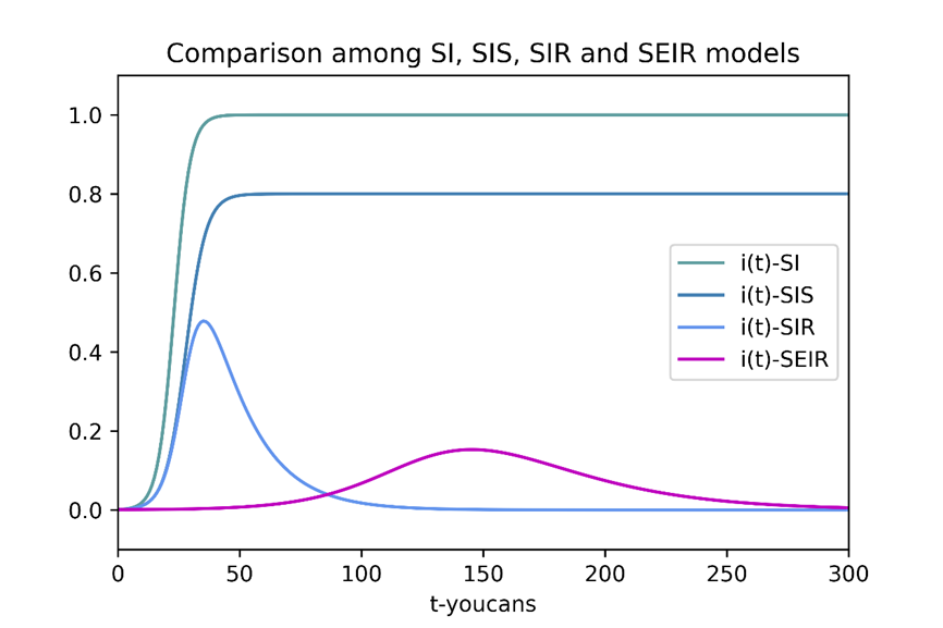
The initial value of the parameter corresponding to the above figure is ：λ=0.3,δ=0.03,μ=0.06,(s0,e0,i0)=(0.001,0.001,0.998), The figure above shows the running result of the routine .
curve i(t)-SI yes SI The result of the model , The proportion of patients has increased sharply to 1.0, All people are infected and become sick , It's not practical .
curve i(t)-SIS yes SIS The result of the model , The proportion of patients increased rapidly and converged to a constant , Steady state eigenvalue i_\infty=1-\mu/\lambda=0.8, It shows that the epidemic situation is stable , And will maintain a certain prevalence rate for a long time .
curve i(t)-SIR yes SIR The result of the model , Proportion of patients i(t) First up to the peak , Then it gradually decreases to a constant .SIR The model can reflect the spread of infectious diseases to some extent , But for infectious diseases with a certain incubation period , Increase as latency E The stage is more in line with the actual situation .
curve i(t)-SEIR yes SEIR The result of the model , Curve and SIR Model i(t) The curve is similar to , The increase reaches the peak and then decreases gradually , Finally tend to 0; However, the proportion curve of patients developed 、 The peak time is later than the latecomer curve , The peak intensity is also low .

Visit alone SEIR The four curves of the model , Infection rate curve and exposure rate curve are basically synchronized , The exposure rate curve is higher than the infection rate curve , Both show a trend of gradually reaching the peak and gradually falling back . The proportion of susceptible people kept decreasing until it fell to 0, Removed by （ The healer and the dead ） The proportion of . overall i(t) and e(t) According to the general law , But the actual transmission process of the actual COVID-19 , The vast majority of people do not become removals after being cured , But always in the susceptible group , Because of the strong control of the government and the self isolation of the residents , Most susceptible people can be isolated from the entire system , This is the case that needs to be considered when modeling .
2. Collect and analyze epidemic data in Shanghai
In the daily epidemic situation announcement published on the official website of the Shanghai Municipal Health Commission , Record key daily data about the epidemic situation , Specifically, it includes new diagnosis 、 New asymptomatic infections 、 Add healing 、 New deaths 、 Those who have been released from quarantine 、 Asymptomatic to confirmed cases 、 Current hospitalized cases and cumulative confirmed cases 、 The most comprehensive epidemic data information such as cumulative cure , It takes a lot of time to make statistics . Due to changes in the caliber of published information and changes in statistical forms , Some data are missing .

Collect the data and conduct statistical analysis , Draw a visual chart to observe the data trend .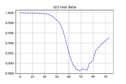

It can be seen from 3 month 1 The trend of each curve from January to the present , Our goal is to make the improved model as close to the real situation as possible .
COVID-19 is an infectious disease with incubation period , The incubation period is usually 2-14 God , It could be longer , So using SEIR The model is more appropriate , But the traditional SEIR The model thinks that in exposed（ Exposed person ） Stage is not contagious , And will only transition to the next stage infected（ infected individual ）, But asymptomatic people infected by the COVID-19 are also infectious , But its complexity lies in that some asymptomatic infected people can turn negative through self-healing , Re entering the susceptible population （susceptible）, So it's different from the traditional SEIR Model .
Apart from self isolation , The rapid flow survey results and the control of close contact groups have greatly reduced the number of effective infectious diseases , However, before and after the implementation of the strict city wide closure measures, there are still great changes in the mobility rate of citizens , Therefore, it is still of great significance for the model to consider the parameter changes before and after strict sealing control . Shanghai from 3 month 28 On the th, Pudong was fully sealed off ,4 month 1 The whole process will be sealed on the th , We take 28 Heaven is the dividing point between the two policies . Refer to the above thinking , Propose improvements SEIR The new model of .
3. The improved SEIR Model

• Parameter interpretation

Parameters	meaning
s	Proportion of susceptible people
e	Proportion of exposed persons
i	Proportion of infected persons
z	Proportion of self isolators
q	Proportion of medical isolators
$\lambda$	Number of daily effective contacts with susceptible people
$\delta$	Daily incidence rate
$\mu$	Daily cure rate
c	Self healing rate of the exposed person
f	Daily self isolation rate
k	Daily medical isolation rate
r	Removal rate of medical isolators
$t_{mark}$	3 month 1 The number of days from January to the beginning of strict sealing control

• Problem modeling
  Modeling the problem with differential equations .
  

• Programming calculation and visualization
  utilize python Modeling solution and visualization , After determining different parameter ranges and carefully adjusting parameters , Basically determine the parameters with good fitting , And draw the trend track of different groups in more than two months , Look for patterns .
  lamda=2,delta=0.15,mu=0.3,tEnd=78,i0=2e-5,e0=2e-5,q0=0,z0= 5e-2,c = 0.3,f = 0.3, k=0.3, r=0.2,t_mark = 28
  
  

Interpretation of the results 、 Discussion and management decision-making suggestions

1. Interpretation of the results
   Compare the actual curve with our forecast curve , We compare the self isolators and the remaining susceptible with the actual susceptible , It is consistent with the actual curve trend in the prediction of susceptible people , And the lowest point is 99%, Quite in line with , The disadvantage is that the actual curve is roughly at the beginning of the current epidemic 50 Days later, the susceptible reached the lowest point , Our model is in 30 It reached the lowest point in several days .
   Compare the infection rate curve that can better reflect the real situation 、 Exposure curve , The model can well represent the same trend of the two curves , That is, the peak value is reached at the same time , We predict that the highest number of infected people can be close to 0.2%, Accessible to the exposed 0.5%, The actual situation is the proportion of infected people 0.1%, Proportion of exposed persons 1%, The maximum difference between the two is ten times . On the one hand, our parameters still need to be adjusted , On the other hand, it is difficult for the model to fully represent the real epidemic situation , The factors affecting the epidemic situation cannot be fully expressed , In addition, whether the collected data can fully represent the actual epidemic trend is also worth discussing .
   The removal rate curve eventually tends to 0.85%, Before introducing self isolators , Infectious diseases will continue to spread until everyone becomes a remover , However, when self isolators are introduced, the removal rate basically conforms to the actual situation , Slightly higher than the actual situation .
   overall , By improving the SEIR Model , Join the self isolators and medical isolators , It is proposed that the exposed persons of novel coronavirus have the condition of self-healing and the self-healing rate is introduced , The model can better reflect the actual situation . The overall trend is completely consistent with the development of actual epidemic data , The proportion of each part is relatively good , Especially for the infected and susceptible people, the prediction is basically consistent , This is of great significance for judging the future epidemic development , But the prediction of inflection point deviates from the actual situation . In addition, due to the fixed parameters , Therefore, it may not be able to reflect the development of the actual epidemic situation more sensitively .
2. Sensitivity analysis
   (1).tmark change
   
   

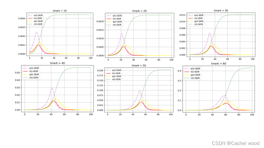
It is of great significance for the development of epidemic situation to strictly control the start time of sealing , From the results of sensitivity analysis, it can be seen that , The epidemic started 10 Day to 20 Days begin to seal , Because the virus has not spread on a large scale , Basically, it can completely inhibit ;30 Days begin to seal , At this time, the infection base for mega cities has been quite large , It is the situation of the outbreak in Shanghai , The medical run is serious , But it's still under control , If the strict sealing control is late 10 Heaven reaches 40 Days later, it will be strictly sealed , Hundreds of thousands or even millions of people will be infected , Then the problem will be very serious . This epidemic has occurred rapidly , Strict containment requires consideration of social costs, citizens and other factors , It needs careful consideration .

(2) Daily self isolation rate f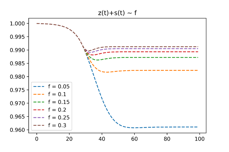

The higher the rate of self isolation , The probability of encountering novel coronavirus is lower , When f>0.2 The proportion of people who are free from novel coronavirus can reach 99%. This isolation rate can be achieved through strong grass-roots mobilization , Therefore, self isolation is a practical means to prevent novel coronavirus .
(3) Daily incidence rate $\delta$

The daily incidence rate mainly depends on the characteristics of the virus and control measures , The incidence rate is controlled at 0.15 Basically, within the controllable range , When the incidence rate is greater than 0.15 Then it will quickly infect a large number of people , The uncontrollable outbreak .

3. Management decision recommendations
   Through the above analysis , Get the following policy recommendations ：

• Government workers need to get confirmed cases quickly 、 Asymptomatic infected persons and close contacts are isolated , The number of effective virus infections has been greatly reduced ;
• Outbreak stage , The government needs to quickly mobilize the general public to isolate themselves , Make the susceptible people in the society in a state of self isolation , Reduce the actual presence of susceptible people , In fact, the number of effective susceptible people should be reduced ;
• The government needs to study and judge the epidemic trend in time , When the epidemic situation becomes more and more serious , A quick judgment must be made between the social cost of strict containment and the spread of the epidemic , Decisively choose extremely strict sealing control measures , Once the best sealing time is missed, the epidemic will spread , The epidemic will become uncontrollable . Of course , Attention must be paid to the accompanying supporting measures .

appendix

• Draw improvements SEIR The model code

	import pandas as pd  
	import matplotlib.colors as mcolors  
	colors=list(mcolors.TABLEAU_COLORS.keys()) # Color change  
	  
	def dySEIR(y, t, lamda, delta, mu, c, f, k, r, tmark):  # SEIR  Model , Derivative function  
	    s, e, i, q, z = y  # youcans 
	  
	    if t<tmark:  
	        ds_dt = -lamda*s*i + c*e  
	        dz_dt = 0  
	    else:  
	        dz_dt = f*s   
	        ds_dt = -lamda*s*i + c*e - f*s # ds/dt = -lamda*s*i 
	    de_dt = lamda*s*i - delta*e - c*e # de/dt = lamda*s*i - delta*e 
	    di_dt = delta*e - mu*i  # di/dt = delta*e - mu*i 
	    dq_dt = k*i - r*q         
	                  
	    return np.array([ds_dt,de_dt,di_dt,dq_dt,dz_dt])  
	  
	def plotseir(number=1e5,lamda=2,delta=0.15,mu=0.3,tEnd=100,i0=2e-5,e0=2e-5,q0=0,z0= 5e-2,c = 0.3,f = 0.3, k=0.3, r=0.2, tmark=28):  
	    t = np.arange(0.0,tEnd,1)  # (start,stop,step) 
	    s0 = 1-i0-e0-q0-z0  #  Initial value of the proportion of susceptible persons  
	  
	    sigma = lamda / mu  #  The number of contacts during the infection period  
	    fsig = 1-1/sigma  
	    Y0 = (s0, e0, i0, q0, z0)  #  Initial value of differential equations  
	      
	    colors=list(mcolors.TABLEAU_COLORS.keys()) # Color change  
	  
	    for i in range(5,33,5):  
	  
	        delta = i/100  
	        ySEIR = odeint(dySEIR, Y0, t, args=(lamda,delta,mu,c,f,k,r,tmark))  # SEIR  Model  
	        print("lamda={}\tdelta={}\tmu={}\tc={}\tf={}\tk={}\tr={}\ttmark={}".format(lamda,delta,mu,c,f,k,r,tmark))  
	  
	        plt.grid()  
	        #plt.plot(t, ySEIR[:,0], '--', color='blue', label='s(t)-SEIR') 
	        plt.plot(t, ySEIR[:,1], '-.', color='orchid', label='e(t)-SEIR')  
	        plt.plot(t, ySEIR[:,2], '-', color='red', label='i(t)-SEIR')  
	        plt.plot(t, ySEIR[:,3], '-', color='yellow', label='q(t)-SEIR')  
	        plt.plot(t, 1-ySEIR[:,0]-ySEIR[:,1]-ySEIR[:,2]-ySEIR[:,3]-ySEIR[:,4], ':', color='green', label='r(t)-SEIR')  
	  
	        #plt.text(0.02,0.36,f"tmark = {tmark}",color='black') 
	        plt.legend(loc='best')  # youcans 
	        plt.title(f'delta = {
      delta}')  
	        plt.savefig(f'eiqr-delta = {
      delta}.png',dpi=600)  
	        plt.show()  
	  
	    for i in range(5,33,5):  
	        delta = i/100  
	        j = i/5-1  
	  
	        plt.grid()  
	  
	        # odeint  Numerical solution , Solving initial value problems of differential equations  
	        ySEIR = odeint(dySEIR, Y0, t, args=(lamda,delta,mu,c,f,k,r,tmark))  # SEIR  Model  
	  
	        print("lamda={}\tdelta={}\tmu={}\tc={}\tf={}\tk={}\tr={}\ttmark={}\t".format(lamda,delta,mu,c,f,k,r,tmark))  
	        #plt.plot(t, ySEIR[:,4], '-', color='pink', label='z(t)-SEIR') 
	        #plt.plot(t, ySEIR[:,0], '--', color='blue', label='s(t)-SEIR') 
	        plt.plot(t,ySEIR[:,0]+ySEIR[:,4],'--',label = f'delta = {
      delta}')  
	    plt.legend()  
	    plt.title('z(t)+s(t) ~ delta')  
	    plt.savefig(f'delta = {
      delta}.png',dpi=600)  
	    plt.show()    
	  
	plotseir()    

• Draw actual data curve code

	df = pd.read_excel('SEIR.xlsx')  
	plt.grid()  
	  
	#plt.subplot(211) 
	plt.plot(df.iloc[:,-4], '--', color='blue', label=df.columns[-4])  
	plt.title('s(t)-real data')  
	plt.savefig('s(t).png',dpi=600)  
	plt.show()  
	  
	#plt.subplot(212) 
	plt.grid()  
	plt.plot(df.iloc[:,-2], '-', color='red', label=df.columns[-2])  
	plt.plot(df.iloc[:,-3], '-.', color='orchid', label=df.columns[-3])  
	plt.plot(df.iloc[:,-1],':', color='green', label=df.columns[-1])  
	plt.legend()  
	plt.title('e(t) i(t) r(t)-real data')  
	  
	plt.savefig('real.png',dpi=600)