Pytorch visualization

One , Visual network structure

In order to conveniently and intuitively view the structure of deep neural network , Generally, the network structure is viewed in a visual way . This section describes how to use torchinfo To visualize the network structure .

1, Use print Function to print the basic information of the model

In this section , We will use ResNet18 Show the structure of ：

import torchvision.models as models
model = models.resnet18()

Go through the two steps above , We get it resnet18 Model structure of . I'm learning torchinfo Before , Let's take a look at the direct print(model) Result ：

ResNet(
  (conv1): Conv2d(3, 64, kernel_size=(7, 7), stride=(2, 2), padding=(3, 3), bias=False)
  (bn1): BatchNorm2d(64, eps=1e-05, momentum=0.1, affine=True, track_running_stats=True)
  (relu): ReLU(inplace=True)
  (maxpool): MaxPool2d(kernel_size=3, stride=2, padding=1, dilation=1, ceil_mode=False)
  (layer1): Sequential(
    (0): Bottleneck(
      (conv1): Conv2d(64, 64, kernel_size=(1, 1), stride=(1, 1), bias=False)
      (bn1): BatchNorm2d(64, eps=1e-05, momentum=0.1, affine=True, track_running_stats=True)
      (conv2): Conv2d(64, 64, kernel_size=(3, 3), stride=(1, 1), padding=(1, 1), bias=False)
      (bn2): BatchNorm2d(64, eps=1e-05, momentum=0.1, affine=True, track_running_stats=True)
      (conv3): Conv2d(64, 256, kernel_size=(1, 1), stride=(1, 1), bias=False)
      (bn3): BatchNorm2d(256, eps=1e-05, momentum=0.1, affine=True, track_running_stats=True)
      (relu): ReLU(inplace=True)
      (downsample): Sequential(
        (0): Conv2d(64, 256, kernel_size=(1, 1), stride=(1, 1), bias=False)
        (1): BatchNorm2d(256, eps=1e-05, momentum=0.1, affine=True, track_running_stats=True)
      )
    )
   ... ...
  )
  (avgpool): AdaptiveAvgPool2d(output_size=(1, 1))
  (fc): Linear(in_features=2048, out_features=1000, bias=True)
)

We can find simple print(model), Only the information of basic components can be obtained , It can't show the of each layer shape, The size of the corresponding parameter quantity cannot be displayed , have access to torchinfo Solve this problem .

2, Use torchinfo Visual network structure

install ：

#  Installation method 1 
pip install torchinfo 
#  Installation method II 
conda install -c conda-forge torchinfo

Use ： Just use **torchinfo.summary()** That's it , The required parameters are model,input_size[batch_size,channel,h,w], For more information, please refer to the link :https://github.com/TylerYep/torchinfo#documentation
Examples are as follows ：

import torchvision.models as models
from torchinfo import summary
resnet18 = models.resnet18() #  Instantiation model 
summary(resnet18, (1, 3, 224, 224)) # 1：batch_size 3: The number of channels in the picture  224:  The height and width of the picture 

Output ：torchinfo Provides more detailed information , Including module information （ The type of each floor 、 Output shape And parameter quantities ）、 The parameter quantity of the whole model 、 The model size 、 Memory size required for a forward or reverse propagation, etc .

Two ,CNN visualization

Convolutional neural networks （CNN） It is a very important model structure in deep learning , but CNN It's a Black box model , People don't know CNN How to get better performance , This brings the interpretability of deep learning .
If you can understand CNN The way we work , People can not only explain the results obtained , Improve the robustness of the model , And it can be targeted to improve CNN To further improve the effect .
understand CNN An important step is visualization , Including how visual features are extracted 、 The form of the extracted features and the concerns of the model in the input data .

1,CNN Convolution kernel Visualization

Convolution kernel at CNN Is responsible for extracting features , Visual convolution kernel can help people understand CNN What features are extracted from each layer , Then understand the working principle of the model . For example, in Zeiler and Fergus 2013 Year of paper I studied it in CNN The convolution kernel of each layer is different , They found that The feature extracted from the layer close to the input is a relatively simple structure , The feature extracted from the layer close to the output is similar to the shape of the entity in the graph .
stay PyTorch It is also very convenient to visualize convolution kernel in , The core lies in the convolution kernel of a specific layer, that is, the model weight of a specific layer , The visual convolution kernel is equivalent to the weight matrix corresponding to the visualization . The following is given in PyTorch Implementation scheme of visual convolution kernel in , With torchvision Self contained VGG11 The model, for example .
First , Load model , And determine the layer information of the model ：

import torch
from torchvision.models import vgg11

model = vgg11(pretrained=True)
print(dict(model.features.named_children()))

{
    '0': Conv2d(3, 64, kernel_size=(3, 3), stride=(1, 1), padding=(1, 1)),
 '1': ReLU(inplace=True),
 '2': MaxPool2d(kernel_size=2, stride=2, padding=0, dilation=1, ceil_mode=False),
 '3': Conv2d(64, 128, kernel_size=(3, 3), stride=(1, 1), padding=(1, 1)),
 '4': ReLU(inplace=True),
 '5': MaxPool2d(kernel_size=2, stride=2, padding=0, dilation=1, ceil_mode=False),
 '6': Conv2d(128, 256, kernel_size=(3, 3), stride=(1, 1), padding=(1, 1)),
 '7': ReLU(inplace=True),
 '8': Conv2d(256, 256, kernel_size=(3, 3), stride=(1, 1), padding=(1, 1)),
 '9': ReLU(inplace=True),
 '10': MaxPool2d(kernel_size=2, stride=2, padding=0, dilation=1, ceil_mode=False),
 '11': Conv2d(256, 512, kernel_size=(3, 3), stride=(1, 1), padding=(1, 1)),
 '12': ReLU(inplace=True),
 '13': Conv2d(512, 512, kernel_size=(3, 3), stride=(1, 1), padding=(1, 1)),
 '14': ReLU(inplace=True),
 '15': MaxPool2d(kernel_size=2, stride=2, padding=0, dilation=1, ceil_mode=False),
 '16': Conv2d(512, 512, kernel_size=(3, 3), stride=(1, 1), padding=(1, 1)),
 '17': ReLU(inplace=True),
 '18': Conv2d(512, 512, kernel_size=(3, 3), stride=(1, 1), padding=(1, 1)),
 '19': ReLU(inplace=True),
 '20': MaxPool2d(kernel_size=2, stride=2, padding=0, dilation=1, ceil_mode=False)}

Convolution kernel corresponds to convolution layer （Conv2d）, Here is the first “3” Layer as an example , Visualize the corresponding parameters ：

conv1 = dict(model.features.named_children())['3']
kernel_set = conv1.weight.detach()
num = len(conv1.weight.detach())
print(kernel_set.shape)
for i in range(0,num):
    i_kernel = kernel_set[i]
    plt.figure(figsize=(20, 17))
    if (len(i_kernel)) > 1:
        for idx, filer in enumerate(i_kernel):
            plt.subplot(9, 9, idx+1) 
            plt.axis('off')
            plt.imshow(filer[ :, :].detach(),cmap='bwr')

torch.Size([128, 64, 3, 3])

Due to the first “3” The characteristic diagram of the layer is composed of 64 Dimension becomes 128 dimension , So there is 128*64 Convolution kernels , The visualization effect of some convolution kernels is shown in the figure below ：

2,CNN Visualization method of feature map

Corresponding to the convolution kernel , The data obtained by each convolution layer of the input original image is called Characteristics of figure , The purpose of visual convolution kernel is to see what features the model extracts , The visual feature map is to see what the features extracted by the model look like .

There are many ways to obtain feature maps , You can start with input , Forward propagation layer by layer , Return it to the desired feature map . Although this method is feasible , But there's some trouble . stay PyTorch in , A special interface is provided to enable the network to obtain the feature map in the process of forward propagation , The name of this interface is very vivid , be called hook. You can imagine a scene like this , Data travels forward through the network , At a certain layer of the network, we preset a hook , After data transmission, the hook will leave the appearance of data in this layer , Reading the information of the hook is the characteristic diagram of this layer . The specific implementation is as follows ：

class Hook(object):
    def __init__(self):
        self.module_name = []
        self.features_in_hook = []
        self.features_out_hook = []

    def __call__(self,module, fea_in, fea_out):
        print("hooker working", self)
        self.module_name.append(module.__class__)
        self.features_in_hook.append(fea_in)
        self.features_out_hook.append(fea_out)
        return None
    

def plot_feature(model, idx, inputs):
    hh = Hook()
    model.features[idx].register_forward_hook(hh)
    
    # forward_model(model,False)
    model.eval()
    _ = model(inputs)
    print(hh.module_name)
    print((hh.features_in_hook[0][0].shape))
    print((hh.features_out_hook[0].shape))
    
    out1 = hh.features_out_hook[0]

    total_ft  = out1.shape[1]
    first_item = out1[0].cpu().clone()    

    plt.figure(figsize=(20, 17))
    

    for ftidx in range(total_ft):
        if ftidx > 99:
            break
        ft = first_item[ftidx]
        plt.subplot(10, 10, ftidx+1) 
        
        plt.axis('off')
        #plt.imshow(ft[ :, :].detach(),cmap='gray')
        plt.imshow(ft[ :, :].detach())

Here we first implement a hook class , After the plot_feature Function , Will be hook Class is registered in a layer of the network to be visualized .model When forward propagation is carried out, it will call hook Of __call__ function , That's where we store the input and output of the current layer . there features_out_hook It's a list, One forward propagation at a time , Are called once , That is to say features_out_hook The length will increase 1

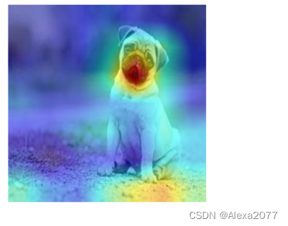
3,CNN class activation map Visualization methods

**class activation map（CAM）** The function of is to judge which variables are important to the model , stay CNN Visual scene , That is, it is important to judge which pixels in the image are important to the prediction result . In addition to identifying important pixels , People will also be interested in the gradient of important areas , So in CAM It has also been further improved on the basis of Grad-CAM（ And many variants ）.CAM and Grad-CAM An example of is shown in the figure below ：

Compared with visual convolution kernel and visual feature graph ,CAM Series visualization is more intuitive , Be able to identify important areas at a glance , Then interpretability analysis or model optimization and improvement .CAM A series of operations can be implemented through the Open Source Toolkit pytorch-grad-cam To achieve .
install ：

pip install grad-cam

routine ：

import torch
from torchvision.models import vgg11,resnet18,resnet101,resnext101_32x8d
import matplotlib.pyplot as plt
from PIL import Image
import numpy as np

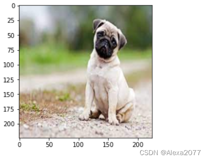
model = vgg11(pretrained=True)
img_path = './dog.png'
# resize The operation is to be consistent with the size of the training picture of the afferent neural network 
img = Image.open(img_path).resize((224,224))
#  You need to convert the original picture to np.float32 Format and in 0-1 Between  
rgb_img = np.float32(img)/255
plt.imshow(img)

from pytorch_grad_cam import GradCAM,ScoreCAM,GradCAMPlusPlus,AblationCAM,XGradCAM,EigenCAM,FullGrad
from pytorch_grad_cam.utils.model_targets import ClassifierOutputTarget
from pytorch_grad_cam.utils.image import show_cam_on_image

target_layers = [model.features[-1]]
#  Select the appropriate class activation diagram , however ScoreCAM and AblationCAM need batch_size
cam = GradCAM(model=model,target_layers=target_layers)
targets = [ClassifierOutputTarget(preds)]   
#  upper preds Need to set , such as ImageNet Yes 1000 class , This can be set to 200
grayscale_cam = cam(input_tensor=img_tensor, targets=targets)
grayscale_cam = grayscale_cam[0, :]
cam_img = show_cam_on_image(rgb_img, grayscale_cam, use_rgb=True)
print(type(cam_img))
Image.fromarray(cam_img)

4, Use FlashTorch Fast implementation CNN visualization

Open source tools are quickly implemented CNN visualization ：FlashTorch:https://github.com/MisaOgura/flashtorch
install ：

pip install flashtorch

Visual gradient ：

# Download example images
# !mkdir -p images
# !wget -nv \
# https://github.com/MisaOgura/flashtorch/raw/master/examples/images/great_grey_owl.jpg \
# https://github.com/MisaOgura/flashtorch/raw/master/examples/images/peacock.jpg \
# https://github.com/MisaOgura/flashtorch/raw/master/examples/images/toucan.jpg \
# -P /content/images

import matplotlib.pyplot as plt
import torchvision.models as models
from flashtorch.utils import apply_transforms, load_image
from flashtorch.saliency import Backprop

model = models.alexnet(pretrained=True)
backprop = Backprop(model)

image = load_image('/content/images/great_grey_owl.jpg')
owl = apply_transforms(image)

target_class = 24
backprop.visualize(owl, target_class, guided=True, use_gpu=True)

Visualization convolution kernel ：

import torchvision.models as models
from flashtorch.activmax import GradientAscent

model = models.vgg16(pretrained=True)
g_ascent = GradientAscent(model.features)

# specify layer and filter info
conv5_1 = model.features[24]
conv5_1_filters = [45, 271, 363, 489]

g_ascent.visualize(conv5_1, conv5_1_filters, title="VGG16: conv5_1")

Reference resources ：
【1】https://andrewhuman.github.io/cnn-hidden-layout_search
【2】https://cloud.tencent.com/developer/article/1747222
【3】https://github.com/jacobgil/pytorch-grad-cam
【4】https://github.com/MisaOgura/flashtorch

3、 ... and , Use TensorBoard Visualize the training process

Use TensorBoard Visualize the training process , Be treated as a separate article ,
The article links ：https://blog.csdn.net/Alexa_/article/details/125940977

This paper is about DataWhale- Explain profound theories in simple language Pytorch Group study notes ！