Model Trick | CVPR 2022 Oral - Stochastic Backpropagation A Memory Efficient Strategy

CVPR 2022 Oral - Stochastic Backpropagation A Memory Efficient Strategy for Training Video Models

This article has authorized the polar market platform , It was launched on the official account of Jishi platform . No second reprint is allowed without permission .

This article is CVPR 2022 ORAL. This paper designs a memory optimization strategy for video task training . actually , This idea can be seen as right from a certain point of view 18 Year paper Backdrop: Stochastic Backpropagation An extension and practicability of the random reverse gradient described in . Next, I will introduce the motivation and details of this method in combination with my personal thinking .

• Original document link （ The content is closer to the original paper ）：https://www.yuque.com/lart/papers/xu5t00
• The paper ：https://arxiv.org/abs/2203.16755

The problem background

There are many training paradigms in video tasks , Of course, this is also related to the target task . For example, what I know , The task of video target segmentation usually randomly samples different video segments （clip） Into the model . The model processes one fragment at a time , Instead of the entire video being sent continuously into the model for processing . Even some video tasks are completely trained according to the image , Just use optical flow to correlate timing information . This paper mainly discusses another kind of , That is, the tasks of video understanding , For example, action recognition 、 Time action positioning and online action detection, etc . These tasks usually rely on video long-term context information . At this time, the problem of insufficient video memory is particularly prominent , This also provides a huge obstacle to the design of end-to-end training .

The common models in this kind of video task can be classified into two types ： Tree model and graph model .

• Tree model ： For long video tasks such as online motion detection and offline motion detection , Most existing methods are Spatial-then-Temporal (StT) Model , That is, most of them are based on an independent system for processing spatial information CNN（2D or 3D-CNN） To extract frames / Characteristics of fragments , Then through an additional time model （RNN,Transformer etc. ） Build context relevance in time . The main feature of this kind of methods is that the extraction process of spatial features is independent .
• Graph model ： What has attracted much attention recently Transformer Is a typical example . In some short-term video tasks , For example, in behavior recognition , Although they have also achieved good results , However, its computing cost and memory occupation also limit its application . The main feature of this kind of method is that the extraction process of spatial features of each frame is an interleaving process .

Therefore, this paper mainly focuses on the improvement of the training process of these two methods , More specifically , Mainly aimed at StT Class methods and Video Transformer Optimization of class methods .

Existing strategies

Video memory optimization strategy of typical video methods

For each part , The existing methods mainly have the following strategies ：

• Reduce the gradient of model parameters ：
  • It is mainly based on the features extracted from the original video in advance , This can be seen as freezing backbone In the form of .DaoTAD Frozen its backbone The first two stages of .
• Start by reducing the amount of data ：
  • Compress input size ： stay AFSD Use in 96×96, stay DaoTAD Use in 112×112.

Although such a strategy ensures the method AFSD[Learning salient boundary feature for anchor-free temporal action localization] and DaoTAD[Rgb stream is enough for temporal action detection] The feasibility of end-to-end training , But in terms of the final effect , This also leads to a decline in accuracy . So we still need to find a more suitable solution . And this kind of scheme can avoid freezing backbone And reduce the data resolution to compress the memory occupation .

These are all from the perspective of model training itself , But from another point of view , We should reflect on , Whether the use of all video data is really necessary ？ From the video data itself , It has a high degree of redundancy , This is also the core motivation of many video compression algorithms . How to make full use of these redundancy to compress training parameters is a content worth exploring . Some typical works are mentioned in this paper , It mainly reduces the occupation of video memory by compressing the number of frames ：

• frame dropout: Vatt: Transformers for multimodal self-supervised learning from raw video, audio and text
• early pool: No frame left behind: Full video action recognition
• frame selections: Smart frame selection for action recognition

These active downsampling input frame sequences , Although it can reduce the occupation of video memory caused by massive data , But it also loses the continuity of fine information in the time domain . And the active downsampling input limits them , It can only be used to handle the tasks of video understanding based on the overall video , For those tasks that need frame by frame prediction, they will face great pressure . At the same time, the processing method of video sampling also requires that the moving speed of video content should not be too fast , Otherwise, the key content is easy to be missed , Affect the prediction effect .

And based on Transformer The new method focuses more on the large proportion of calculation cost Attention Redesign and optimization of operations , To strengthen its modeling ability for long sequence tasks .

General video memory compression strategy

• Time for space ：
  • Gradient checkpoint technology [Training deep nets with sublinear memory cost]： Forward propagation no longer preserves gradient information , Back propagation recalculates the correlation gradient , More on PyTorch And Checkpoint Mechanism analysis . The disadvantage is that it will slow down the training speed , Basically does not affect the performance .
  • Gradient accumulation technique ： That is, through multiple forward propagation, a single large batch The effect of , More on PyTorch Why do you need to reset the gradient manually before backpropagation ？ - You know . Will slow down the training speed , Probably because of batch Differences in statistics , But with the truth batch There are differences .
• Other strategies ：
  • Sparse networks [Sparse networks from scratch: Faster training without losing performance] Applied to image recognition model , But it can only save memory in theory .
  • Sideways[Sideways: Depth-parallel training of video models, Gradient forward-propagation for large-scale temporal video modelling] in , Whenever a new activation is available , The original activation will be overwritten , But this can only be applied to causal models . This also reduces memory consumption .

Program motivation

Experimental observation

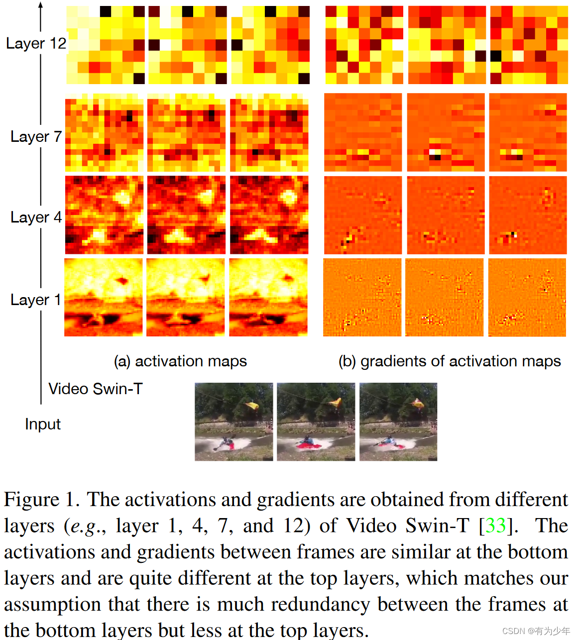
The authors show that in Kinetics-400 Video on Swin Activation diagram and gradient diagram . The authors assume that the complete activation diagram （ In the forward path ） It is necessary to extract important semantic information , But for gradients （ Reverse path ） May be unnecessary . On the diagram, it can be seen visually that the activation diagram and gradient diagram of a specific layer of the model are similar to the shallow layer , But there are deep differences .

In fact, according to the sequence of data generation , The activation diagram is the shallow layer affecting the deep layer , The gradient map is the deep layer affecting the shallow layer , Therefore, we can deduce the author's motivation to delete the shallow structure gradient .

Inspired by relevant methods

This point was raised by me alone , I think these works should have important inspiration for the design of this article , Or it has important reference value for us to understand the motivation of this article .

• Regularizing metalearning via gradient dropout： This work was mentioned by the author . It reduces the ratio by setting zero （10％~20％） To regularize the training process . This article is different , The deletion proportion of this article is larger , And it is mainly used for compressing video memory .
• Vatt: Transformers for multimodal self-supervised learning from raw video, audio and text： This work uses a lightweight network to sample frames from video , Therefore, the forward and reverse paths of the corresponding frame will be deleted at the same time . However, this paper only randomly deletes a certain proportion of back propagation paths , Keep all forward paths at the same time . Complete video information is very important for time modeling .
• Backdrop: Stochastic Backpropagation： This article 18 The work of this paper is also very similar to the article in , Although there is no mention of , But here I think it is necessary to point out .

Backdrop In this work, it is proposed to add drop Operation to improve the efficiency of data utilization , Reduce overfitting . The core operation is very similar to this article , That is, forward propagation is not modified , And just randomly delete some back propagation paths . At the same time, this work is described as follows in the final summary ：

In our initial implementation of backdrop, the blocked gradients are still computed but are simply multiplied by zero. A more efficient implementation, where the gradients are not computed for the blocked paths, would therefore lead to a significant decrease in computation time as well as in memory requirements. In a similar fashion, we would expect backdrop to be a natural addition to gradient checkpointing schemes whose aim is to reduce memory requirements [Training deep nets with sublinear memory cost, Memory-efficient backpropagation through time].

Similar to other tools in a machine-learning toolset, backdrop masking should be used judiciously and after considerations of the structure of the problem. However, it can also be used in autoML schemes where a number of masking layers are inserted and the masking probabilities are then fine-tuned as hyperparameters.

You can see , The work of this paper can be seen as a contribution to Backdrop An extended application of the medium-term expected content in the field of video tasks .(#^.#)

The specific plan

As the previous analysis , The redundancy of gradients in shallow structures , And the independency with deep features , It ensures the feasibility of deleting shallow gradients to compress the occupation of video memory . Therefore, the authors propose a method called random back propagation （SBP） Method for compressing video model video memory occupation .

To be specific , During video model training ,SBP Keep all forward propagation paths , However, in each training step, the back propagation path of each network layer is deleted randomly and independently . Although this operation results in that some parameters in the model cannot be updated due to the destruction of the gradient chain rule , But according to experience , Just keep the overall calculation diagram , The network parameters can still be updated effectively .

It reduces some of the cache requirements corresponding to back propagation , To reduce GPU Storage costs . And this amount can be adjusted by the retention rate （keep-ratio） To control . The ultimate savings depend only on the retention rate , And when it's low , The degree of memory saving is also more significant .

Experiments show that ,SBP Various models that can be applied to video tasks , In the task of action recognition and time action detection , Can save up to 80.0％ Of GPU Storage , And promote 10％ Training speed , And the accuracy dropped by less than 1％.

The practical application

Because there are two kinds of models commonly used in video tasks , The tree model and graph model mentioned above , The specific architecture forms are different , This led to the SBP In application, it needs to be considered separately .

First of all, I will explain what will be mentioned repeatedly in the following text “ node ” The definition of .

When the model is defined , Its back propagation can be seen as a directed acyclic graph （Directed Acyclic Graph (DAG)）, The top of it V Corresponds to the activation of the cache for gradient calculation , And the edge E Are the operations used to calculate the gradient . Because the model can be seen as a stack of different layers , So you can also organize the elements in the vertex in the way of layers , Each element is numbered according to the corresponding layer $l_i$ To divide into multiple $V_{l_i}$.
there $V_{l_i}$ Can represent layers $l_i$ Output , and $V_{l_0}$ Represents the model input .
Every $V_{l_i}$ It can be seen as a set of eigenvectors , for example , If $V_{l_i}$ It's a CxDxHxW The amount of , You can think of it as DxHxW A collection of vertices . Every vertex here （ It is called in the paper “node”）, It's a C The eigenvectors of the dimensions .

The author divides the models to be analyzed into two parts ：1） Spatial model （ Below the dotted line ） and 2） Time model （ Above the dotted line ）.

• The deep structure can be seen as a time model , Because these layers mainly learn global semantic information from all frames .
• Shallow structure is usually regarded as a spatial model that mainly learns spatial and local context information .

A typical feature of tree model is that the bottom layer is responsible for spatial modeling of each frame （ Typical cases are using fixed spaces backbone Extract frame features ）, The top layer is used to combine the information of each frame for time modeling . Due to the redundancy of the spatial model , In actual processing ,SBP Apply only to remove gradients on shallow spatial structures . And it's good to do so , That is, the feature size in the shallow structure is often much larger than that in the deep structure , Therefore, removing the gradient of the former can also avoid tracking the corresponding intermediate nodes , This can save a lot of memory . therefore , The gradient propagates only on the nodes of the reserved reverse path . Moreover, the particularity of this kind of model also leads to the fact that the gradient of the sampling node has nothing to do with whether other nodes are sampled .

There is a strong correlation between nodes in the graph model ,Vision Transformer Is a typical full connection graph model . The graph model will be applied at the layer level SBP, Instead of the spatial model level in the tree model . Back propagation also occurs only between sampled nodes . These characteristics cause the gradient calculation of sampling nodes to become more and more inaccurate with the back propagation process . However, the top-down redundancy of back propagation ensures that such operations will not cause too many problems . However, maintaining the same sampling nodes across layers can also alleviate this problem . The identification of parameters can be simplified by setting a uniform retention rate for all layers . However, a systematic strategy can be developed to set the layer specific retention rate .

Here we show Attention Forms of use in layers . The proposed method will sample the same nodes for all layers （ Grey nodes ）.

Because each query Actually with the whole key and value Have a relationship . So in order to calculate accurately query Gradient of nodes , Here will be reserved for all key and value node . This reservation is negligible compared to the memory occupation of the attention weight obtained by dot multiplication , The latter is the big head .

In order to correspond to the concepts of spatial model and temporal model described above , The authors will Video Transformer The deepest layers in the are used as time models . These parts have a complete back propagation path , and SBP Only in the remaining layers . These layers can be viewed as spatial models .

Concrete realization

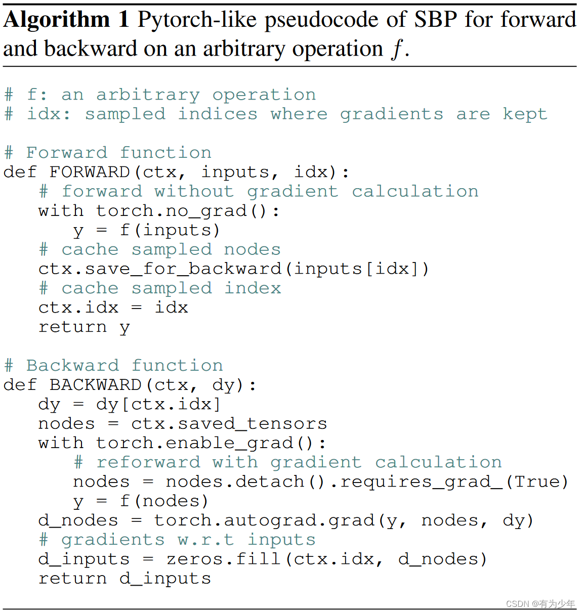
The pseudo code of the algorithm implementation is given in this paper , Any operation here f Both include StT The spatial model in the model also includes Video Transformer Dot multiplication attention and multi-layer perceptron in .

• During forward propagation , The automatic differentiation engine does not track these parameters throughout the operation . Given the sampling index idx Only the input that needs to calculate the gradient is saved , For back propagation .
• During back propagation , Reestablish the gradient path for the returned gradients at the specified sampling location . That is, the forward propagation is performed again on the sampling input and the gradient is returned .

Such an implementation can take full advantage of the automatic differentiation engine , So it's very efficient , There's almost no overhead .

Space and time complexity

A parameter is introduced here , Retention rate r. That is, compared with the number of nodes in the complete gradient path , perform SBP The proportion of the number of nodes that still maintain the gradient calculation .

• StT Space model and time model are independent of each other , also SBP Only works on spatial models . Because the space model in this kind of model often occupies a large space , So execute SBP Compared with the previous occupation, the latter can be approximated as the retention rate r.
• Video Transformer In the model , On the assumption that the dimension of the head of multi - head attention and token The number of them is respectively d and n when , It is necessary to calculate the occupation of the activation graph of the gradient , In the use of SBP The comparison between before and after is as follows , It is approximately proportional to the sampling rate r. therefore r If it's small enough , Memory usage can be significantly reduced .

About the time compression ratio , Suppose the time of forward propagation and back propagation are equal , Then the complete proportion is (1+2r)/2, Because we actually did 1+r Times forward propagation and r Times back propagation .

Experimental results

Similarity measure

In the experiments , The authors introduced Similarity of neural network representations revisited Used to measure the similarity between two neural networks CKA Measure by similarity Video Swin-T The similarity of the same layer activation . The figure shows three training settings and complete end-to-end training （ That is to say “Video Swin”） The similarity of . curve FD（frame dropout） Show the use of 1/4 The model trained by number of frames is the same as the model trained by all frames （ Baseline model “Video Swin”） Between CKA similarity . Look at it from another Angle ,FD The solution is equivalent to removing... From all layers 3/4 Gradient of .

From the figure, we can clearly see the similarity of the shallow structure representation corresponding to the three structures . As far as I can guess , The curve of the graph shown here should correspond to the representation similarity of the training complete model .

so , Use SBP and FD In the model of , Shallow layers have high similarity , The similarity of deep structure is not very high , This also confirms the previous figure 1 Show in , Subtle changes in the characterization of shallow structures can lead to great differences in deep structures . The author believes that after randomly cutting off the backpropagation path , The phenomenon that shallow features still maintain high similarity , This means that discarding a portion of the gradient does not significantly reduce the performance of the model . Use at the same time SBP Method in deep structure CKA Similarity is higher than using FD, The author believes that this also implies the significance of maintaining complete gradient calculation in deep structure .

But what deserves our attention is , It can be seen that such truncation operation has a significant impact on deep features , This doesn't seem to make a huge difference in performance ？ Or to say , Is it because of this difference , As a result, the final performance is still slightly weaker than the complete training ？ On the other hand , It also seems to reflect the close coupling between forward propagation and back propagation , Although in SBP It is completely preserved in the forward propagation , However, the adjustment of back propagation still results in significant differences from the original baseline characterization . It is a pity , The authors did not give more analysis of these .

Behavior recognition

In the experiments SBP Only the shallow time dimension is uniformly and randomly sampled . In this way, the nodes corresponding to the frame can be either sampled or discarded . In all layers , The sampling nodes are consistent .

In contrast ,SBP The best performance is achieved under the trade-off between performance and video memory occupation .
Time dependent data sets （Epic-55） On FD The serious loss of performance also shows the importance of maintaining all forward propagation paths in the process of training and reasoning .

It can be seen from the comparison of gradient Checkpoint Technology ：

• When used alone , The memory consumption of the two is close , however SBP You can make an appointment soon 30%.
• When used together , Compared with using alone SBP, It can save about 40% Memory footprint .

in addition , According to the text , The authors also tested SBP and O1 The matching effect of level mixed accuracy training , Found that this can save Swin-T More than about 50% Of memory , Without performance degradation .

In fact, the three can be used at the same time , But the author did not provide more information about this .

The previous experiments were carried out in the time dimension . All nodes in a frame are either retained or discarded .
The authors added that gradient discarding is performed simultaneously in time and space , Used 3D Spatiotemporal gradient discarding strategy of chessboard mode .
In contrast , Time sampling （ That is, frame level processing ） And spatiotemporal sampling （ namely 3D Chessboard form ） Similar performance . It also reflects SBP Potential for spatial sampling and migration to image domain .

Time behavior detection

In order to verify the performance in long-time video tasks , The authors also verified the time behavior test .

The online motion detection task needs to detect the actions that are happening in each frame in the real-time video stream , Instead of using future information .
Existing methods continue StT normal form , Based on the extracted video frame features, the modeling of timing information is performed on the time model .

In the experiment, we can see ：

• End to end training is better than freezing backbone The strategy of , But video memory takes up a lot more .
• Lower retention r=0.125 Of SBP The final performance is even slightly better than end-to-end training . The author attributes it to SBP Regularization of , Can alleviate over fitting .
• LSTR The improvement is greater than TRN Improvement , This shows that a stronger time model can benefit from end-to-end training .

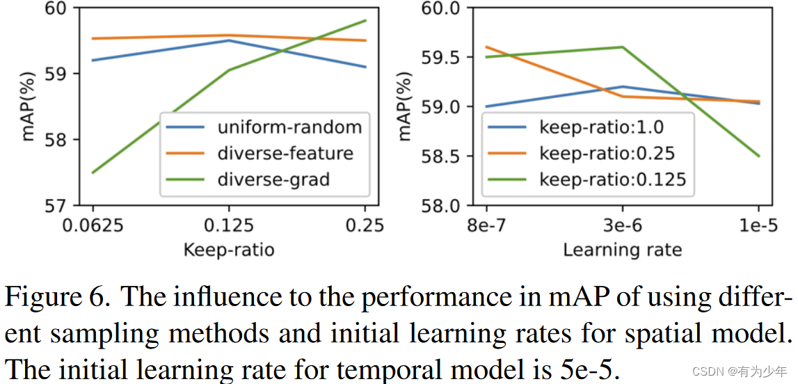
in the light of SBP How to sample nodes , Here's a comparison of three strategies ：

• Uniform Random Sampler： The candidate nodes are evenly divided into multiple nodes along the time dimension chunk in . Every chunk The size is 1/r. Finally in each chunk Randomly sample a node in . This is also the default way .
• Diverse-Feature Sampler： Sort candidate nodes according to amplitude , Then perform uniform random sampling .
• Diverse-Grad Sampler： Rank candidate nodes by amplitude , Then perform uniform random sampling .

From the comparison we can see ：

• diverse-feature sampler Achieved the best overall mAP.
• Three types of sampler mAP Really close , It also reflects the robustness of the method to the sampler .

Because uniform sampling achieves good mAP, And it's simpler , So it is used in all other experiments by default .

The author also makes an experiment on the learning rate of spatial model . For the use of SBP Of StT Model ：

• For all retention rates , The learning rate of the best spatial model is about that of the time model 0.1 About times .
• Use SBP, Spatial models are indeed more robust to learning rates , As long as they are relatively small .
  therefore , If not stated , By default, the learning rate of the spatial model is the same as that of the temporal model 0.1 times .

Time action positioning

Temporal action localization aims to detect the time boundary of each action instance in untrimmed video . Most existing methods follow StT normal form .

In the experiments , End to end training performance is better than freezing backbone Of , But video memory is also much larger . introduce SBP A better trade-off is obtained .

limitations

• First ,SBP Is a new prototype technology , This proves that memory can be saved by discarding the back propagation path , But it also comes with a slight drop in accuracy . Future exploration can focus on more adaptive layer retention and sampling methods , To reduce the loss of accuracy , Even the accuracy is improved due to the regularization effect caused by gradient discarding .
• secondly ,SBP Only a small increase in training speed （~1.1×）. however , How to compare it with other effective model training strategies （ for example Multigrid [A multigrid method for efficiently training video models]） Integrate , To speed up training is still to be explored .